Statistical Graphics and Visualization course materials

I’ve just finished teaching the Fall 2015 session of 36-721, Statistical Graphics and Visualization. Again, it is a half-semester course designed primarily for students in the MSP program (Masters of Statistical Practice) in the CMU statistics department. I’m pleased that we also had a large number of students from other departments taking this as an elective.

For software we used mostly R (base graphics, ggplot2, and Shiny). But we also spent some time on Tableau, Inkscape, D3, and GGobi.

We covered a LOT of ground. At each point I tried to hammer home the importance of legible, comprehensible graphics that respect human visual perception.

Pie chart with remake — Remaking pie charts is a rite of passage for statistical graphics students

My course materials are below. Not all the slides are designed to stand alone, but I have no time to remake them right now. I’ll post some reflections separately.

Download all materials as a ZIP file (38 MB), or browse individual files:
Continue reading “Statistical Graphics and Visualization course materials” →

Summary sheet of ways to map statistical uncertainty

A few years ago, a team at the Cornell Program on Applied Demographics (PAD) created a really nice demo of several ways to show statistical uncertainty on thematic maps / choropleths. They have kindly allowed me to host their large file here: PAD_MappingExample.pdf (63 MB)

Screenshot of index page from PAD mapping examples

Each of these maps shows a dataset with statistical estimates and their precision/uncertainty for various areas in New York state. If we use color or shading to show the estimates, like in a traditional choropleth map, how can we also show the uncertainty at the same time? The PAD examples include several variations of static maps, interaction by toggling overlays, and interaction with mouseover and sliders. Interactive map screenshots are linked to live demos on the PAD website.

I’m still fascinated by this problem. Each of these approaches has its strengths and weaknesses: Symbology Overlay uses separable dimensions, but there’s no natural order to the symbols. Pixelated Classification seems intuitively clear, but may be misleading if people (incorrectly) try to find meaning in the locations of pixels within an area. Side-by-side maps are each clear on their own, but it’s hard to see both variables at once. Dynamic Feedback gives detailed info about precision, but only for one area at a time, not all at once. And so forth. It’s an interesting challenge, and I find it really helpful to see so many potential solutions collected in one document.

The creators include Nij Tontisirin and Sutee Anantsuksomsri (both since moved on from Cornell), and Jan Vink and Joe Francis (both still there). The pixellated classification map is based on work by Nicholas Nagle.

For more about mapping uncertainty, see their paper:

Francis, J., Tontisirin, N., Anantsuksomsri, S., Vink, J., & Zhong, V. (2015). Alternative strategies for mapping ACS estimates and error of estimation. In Hoque, N. and Potter, L. B. (Eds.), Emerging Techniques in Applied Demography (pp. 247–273). Dordrecht: Springer Netherlands, DOI: 10.1007/978-94-017-8990-5_16 [preprint]

and my related posts:

Localized Comparisons: my own attempts at showing uncertainty in an interactive map and in a cartogram, plus links to work by Gabriel Florit, David Sparks, Nicholas Nagle, and Nancy Torrieri & David Wong
Nice example of a map with uncertainty: a map by Michael Wininger

See also Visualizing Attribute Uncertainty in the ACS: An Empirical Study of Decision-Making with Urban Planners. This talk by Amy Griffin is about studying how urban planners actually use statistical uncertainty on maps in their work.

About to teach Statistical Graphics and Visualization course at CMU

I’m pretty excited for tomorrow: I’ll begin teaching the Fall 2015 offering of 36-721, Statistical Graphics and Visualization. This is a half-semester course designed primarily for students in our MSP program (Masters in Statistical Practice).

A large part of the focus will be on useful principles and frameworks: human visual perception, the Grammar of Graphics, graphic design and interaction design, and more current dataviz research. As for tools, besides base R and ggplot2, I’ll introduce a bit of Tableau, D3.js, and Inkscape/Illustrator. For assessments, I’m trying a variant of “specs grading”, with a heavy use of rubrics, hoping to make my expectations clear and my TA’s grading easier.

Di Cook, LDA and CART classification boundaries on Flea Beetles dataset — Classifier diagnostics from Cook & Swayne’s book

My initial course materials are up on my department webpage.
Here are the

syllabus (pdf),
first lecture (pdf created with Rmd), and
first homework (pdf) with dataset (csv).

(I’ll probably just use Blackboard during the semester, but I may post the final materials here again.)

It’s been a pleasant challenge to plan a course that can satisfy statisticians (slice and dice data quickly to support detailed analyses! examine residuals and other model diagnostics! work with data formats from rectangular CSVs through shapefiles to social networks!) … while also passing on lessons from the data journalism and design communities (take design and the user experience seriously! use layout, typography, and interaction sensibly!). I’m also trying to put into practice all the advice from teaching seminars I’ve taken at CMU’s Eberly Center.

Also, in preparation, this summer I finally enjoyed reading more of the classic visualization books on my list.

Cleveland’s The Elements of Graphing Data and Robbins’ Creating More Effective Graphs are chock full of advice on making clear graphics that harness human visual perception correctly.
Ware’s Information Visualization adds to this the latest research findings and a ton of useful detail.
Cleveland’s Visualizing Data and Cook & Swayne’s Interactive and Dynamic Graphics for Data Analysis are a treasure trove of practical data analysis advice. Cleveland’s many case studies show how graphics are a critical part of exploratory data analysis (EDA) and model-checking. In several cases, his analysis demonstrates that previously-published findings used an inappropriate model and reached poor conclusions due to what he calls rote data analysis (RDA). Cook & Swayne do similar work with more modern statistical methods, including the first time I’ve seen graphical diagnostics for many machine learning tools. There’s also a great section on visualizing missing data. The title is misleading: you don’t need R and GGobi to learn a lot from their book.
Monmonier’s How to Lie with Maps refers to dated technology, but the concepts are great. It’s still useful to know just how maps are made, and how different projections work and why it matters. Much of cartographic work sounds analogous to statistical work: making simplifications in order to convey a point more clearly, worrying about data quality and provenance (different areas on the map might have been updated by different folks at different times), setting national standards that are imperfect but necessary… The section on “data maps” is critical for any statistician working with spatial data, and the chapter on bureaucratic mapping agencies will sound familiar to my Census Bureau colleagues.

I hope to post longer notes on each book sometime later.

Dataviz contest on “Visualizing Well-Being”

Someone from OECD emailed me about a data visualization contest for the Wikiprogress website (the deadline is August 24th):

I am contacting you on behalf of the website Wikiprogress, which is currently running a Data Visualization Contest, with the prize of a paid trip to Mexico to attend the 5th OECD World Forum in Guadalajara in October this year. Wikiprogress is an open-source website, hosted by the OECD, to facilitate the exchange of information on well-being and sustainability, and the aim of the competition is to encourage participants to use well-being measurement in innovative ways to a) show how data on well-being give a more meaningful picture of the progress of societies than more traditional growth-oriented approaches, and b) to use their creativity to communicate key ideas about well-being to a broad audience.

After reading your blog, I think that you and your readers might be interested in this challenge. The OECD World Forums bring together hundreds of change-makers from around the world, from world leaders to small, grassroots projects, and the winners will have their work displayed and will be presented with a certificate of recognition during the event.

You can also visit the competition website here: http://bit.ly/1Gsso2y

It does sound like a challenge that might intrigue this blog’s readers:

think about how to report human well-being, beyond traditional measures like GDP;
find relevant good datasets (“official statistics” or otherwise);
visualize these measures’ importance or insightful trends in the data; and
possibly win a prize trip to the next OECD forum in Guadalajara, Mexico to network with others who are interested in putting data, statistics, and visualization to good use.

Two principled approaches to data visualization

Yesterday I spoke at Stat Bytes, our student-run statistical computing seminar.

My goal was to introduce two principled frameworks for thinking about data visualization: human visual perception and the Grammar of Graphics.
(We also covered some relevant R packages: RColorBrewer, directlabels, and a gentle intro to ggplot2.)

These are not the only “right” approaches, nor do they guarantee your graphics will be good. They are just useful tools to have in your arsenal.

Example plot with direct labels and ColorBrewer colors, made in ggplot2.

The talk was also a teaser for my upcoming fall course, 36-721: Statistical Graphics and Visualization [draft syllabus pdf].

Here are my

The talk was quite interactive, so the slides aren’t designed to stand alone. Open the slides and follow along using my notes below.
(Answers are intentionally in white text, so you have a chance to think for yourself before you highlight the text to read them.)

If you want a deeper introduction to dataviz, including human visual perception, Alberto Cairo’s The Functional Art [website, amazon] is a great place to start.
For a more thorough intro to ggplot2, see creator Hadley Wickham’s own presentations at the bottom of this page.

Continue reading “Two principled approaches to data visualization” →

Nice example of a map with uncertainty

OK, back to statistics and datavis.

As I’ve said before, I’m curious about finding better ways to draw maps which simultaneously show numerical estimates and their precision or uncertainty.

The April 2015 issue of Significance magazine includes a nice example of this [subscription link; PDF], thanks to Michael Wininger. Here is his Figure 2a (I think the labels for the red and blue areas are mistakenly swapped, but you get the idea):

Basically, Wininger is mapping the weather continuously over space, and he overlays two contours: one for where the predicted snowfall amount is highest, and another for where the probability of snowfall is highest.

I can imagine people would also enjoy an interactive version of this map, where you have sliders for the two cutoffs (how many inches of snow? what level of certainty?). You could also just show more levels of the contours on one static map, by adding extra lines, though that would get messy fast.

I think Wininger’s approach looks great and is easy to read, but it works largely because he’s mapping spatially-continuous data. The snowfall levels and their certainties are estimated at a very fine spatial resolution, unlike say a choropleth map of the average snowfall by county or by state. The other thing that helps here is that certainty is expressed as a probability (which most people can interpret)… not as a measure of spread or precision (standard deviation, margin of error, coefficient of variation, or what have you).

Could this also work on a choropleth map? If you only have data at the level of discrete areas, such as counties… Well, this is not a problem with weather data, but it does come up with administrative or survey data. Say you have survey estimates for the poverty rate in each county (along with MOEs or some other measure of precision). You could still use one color to fill all the counties with high estimated poverty rates. Then use another color to fill all the counties with highly precise estimates. Their overlap would show the areas where poverty is estimated to be high and that estimate is very precise. Sliders would let the readers set their own definition of “high poverty” and “highly precise.”

I might be wrong, but I don’t think I’ve seen this approach before. Could be worth a try.

Dataclysm, Christian Rudder

In between project deadlines and homework assignments, I enjoyed taking a break to read Christian Rudder’s Dataclysm. (That’s right, my pleasure-reading break from statistics grad school textbooks is… a different book about statistics. I think I have a problem. Please suggest some good fiction!)

So, Rudder is one of the founders of dating site OkCupid and its quirky, data-driven research blog. His new book is very readable—each short, catchy chapter was hard to put down. I like how he gently alludes to the statistical details for nerds like myself, in a way that shouldn’t overwhelm lay readers. The clean, Tufte-minimalist graphs work quite well and are accompanied by clear writeups. Some of the insights are basically repeats of material already on the blog, but with a cleaner writeup, though there’s plenty of new stuff too. Whether or not you agree with all of his conclusions [edit: see Cathy O’Neil’s valid critiques of the stats analyses here], the book sets a good example to follow for anyone interested in data- or evidence-based popular science writing.

Most of all, I loved his description of statistical precision:

Ironically, with research like this, precision is often less appropriate than a generalization. That’s why I often round findings to the nearest 5 or 10 and the words ‘roughly’ and ‘approximately’ and ‘about’ appear frequently in these pages. When you see in some article that ‘89.6 percent’ of people do x, the real finding is that ‘many’ or ‘nearly all’ or ‘roughly 90 percent’ of them do it, it’s just that the writer probably thought the decimals sounded cooler and more authoritative. The next time a scientist runs the numbers, perhaps the outcome will be 85.2 percent. The next time, maybe it’s 93.4. Look out at the churning ocean and ask yourself exactly which whitecap is ‘sea level.’ It’s a pointless exercise at best. At worst, it’s a misleading one.

I might use that next time I teach.

The description of how academics hunt for data is also spot on: “Data sets move through the research community like yeti—I have a bunch of interesting stuff but I can’t say from where; I heard someone at Temple has tons of Amazon reviews; I think L has a scrape of Facebook.”

Sorry I didn’t take many notes this time, but Alberto Cairo’s post on the book links to a few more detailed reviews.

Winter is coming (to the Broad Street pump)

We live in an amazing future, where an offhand Twitter joke about classic data visualizations and Game of Thrones immediately turns into a real t-shirt you can buy.

Hats off to Alberto Cairo (whose book The Functional Art and blog are the best introductions to data visualization that I can recommend—but you already knew that).

If you don’t already know the story of John Snow and the Broad Street pump—or if you think you do but haven’t heard the full details—then The Ghost Map is a great telling.

Update: Alberto continues to kick this up a notch, adding two more Game Of Thrones-themed classic dataviz jokes, and making the images/captions available under the Creative Commons license. Awesome.

‘Census Marketing’ app by Olin College students

I love having the chance to promote nifty data visualizations; good work from my former employer, the Census Bureau; and student projects from my alma mater, Olin College. So it’s a particular pleasure to highlight all three at once:

Elizabeth Duncan and Marena Richardson, students in Olin’s Data Science course, teamed up with Census staff and BusinessUSA to develop an app that helps make Census data accessible to small business owners.

The result, Census Marketing, is a nifty and simple interface to overlay Decennial Census and American Community Survey data on Google Maps.

Imagine you’re planning to start or expand a small business, and you know the demographic you’d like to target (age, income, etc.) Where in your town is there a high concentration of your target market? And, are there already competing businesses nearby?

Load up Duncan and Richardson’s website, enter your location, select demographic categories from a few drop-down menus, and give your business type. The app will go find the relevant data (through the Census API) and display it for you as a block-level heatmap on Google Maps. It’ll also highlight the locations of existing businesses that might be competitors.

For example, say you want to open a pizzeria in my Pittsburgh neighborhood of Squirrel Hill. You might want to target the undergrad and grad student populations, since they tend to order pizza pretty often. Punch in the zip code 15217, choose all races and both sexes, select age groups 20-29 and 30-39, and specify that you’re looking for other competing pizzerias:

Well! The student-age population is clearly concentrated around Hobart and Murray… but so are the competing pizzerias. Good to know. Maybe you need to brainstorm a new business plan, seek out a different part of town, or try marketing to a different demographic.

Besides learning about data science and creating a website, Duncan and Richardson also interviewed several actual small business owners to refine the user experience. It’s a nice example of Olin’s design-centered approach to engineering education. I can imagine a couple of further improvements to this app… But it’s already a nice use case for the Census API, and a good example of the work Olin students can do in a short time.

PS—the course instructor, Allen Downey, has a free book ThinkStats on introductory statistics from a computer scientist’s point of view. I hear that a revised second edition is on its way.

Data-Driven Journalism MOOC

TL;DR: The Knight Center’s free online journalism courses are great for anyone who works with data, storytelling, or both. See what’s being offered here.
My favorite links from a recent course on Data-Driven Journalism are here.
And a fellow student’s suggested reading list is here.

Last fall, a coworker and I led a study group for the Knight Center‘s MOOC (massive open online course) on “Introduction to Infographics and Data Visualization”, taught by Alberto Cairo. The course and Alberto’s book were excellent, and we were actually able to bring Alberto in to the Census Bureau for a great lecture a few months later. This course is now in its 3rd offering (starting today!) and I cannot recommend it highly enough if you have any interest in data, journalism, visualization, design, storytelling, etc.!

So, this summer I was happy to see the Knight Center offering another MOOC, this time on “Data-Driven Journalism: The Basics”. What with moving cities and starting the semester, I hadn’t kept up with the class, but I’ve finally finished the last few readings & videos. Overall I found a ton of great material.

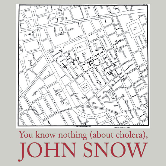
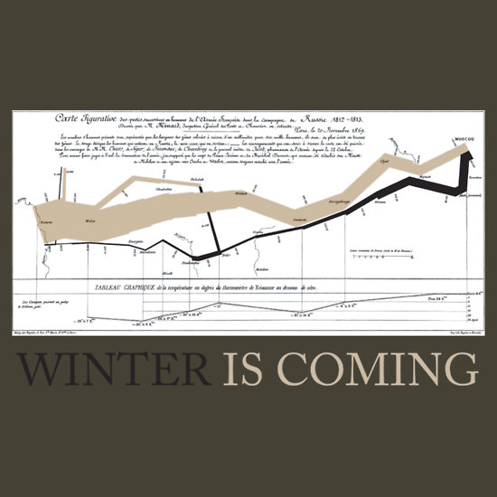
The course’s five lecturers gave an overview of data-driven journalism: from its historical roots in the 1800s and its relation to computer-aided reporting, to how to get data in the first place, through cleaning and checking the data, and finally to building news apps and journalistic data visualizations.

In week 3 there was a particularly useful exercise of going through a spreadsheet of hunting accidents. Of course it illustrated some of the difficulties in cleaning data, and it gave concrete practice in filtering and sorting. But it was also a great illustration of how a database can lead you potential trends or stories that you might have missed if you’d only gone out to interview a few individual hunters.

I loved some of the language that came up, such as “backgrounding the data” — analogous to checking out your sources to see how much you can trust them — or “interrogating the data,” including coming prepared to the “data interview” to ask thorough, thoughtful questions. I’d love to see a Statistics 101 course taught from this perspective. Statisticians do these things all the time, but our terminology and approach seem alien and confusing the first few times you see them. “Thinking like a journalist” and “thinking like a statistician” are not all that different, and the former might be a much more approachable path to the latter.

For those who missed the course, consider skimming the Data Journalism Handbook (free online); Stanford’s Data Journalism lectures (hour-long video); the course readings I saved on Pinboard; and my notes below.
Edit: See also fellow student Daniel Drew Turner’s suggested reading list.
Then, keep an eye out for next time it’s offered on the Knight Center MOOC page.

Below is a (very messy) braindump of notes I took during the class, in case there are any useful nuggets in there. (Messiness due to my own limited time to clean the notes up, not to any disorganization in the course itself!) I think the course videos were not for sharing outside the class, but I’ve linked to the other readings and videos.

Continue reading “Data-Driven Journalism MOOC” →