“Don’t invert that matrix” – why and how

The first time I read John Cook’s advice “Don’t invert that matrix,” I wasn’t sure how to follow it. I was familiar with manipulating matrices analytically (with pencil and paper) for statistical derivations, but not with implementation details in software. For reference, here are some simple examples in MATLAB and R, showing what to avoid and what to do instead.

[Edit: R code examples and results have been revised based on Nicholas Nagle’s comment below and advice from Ryan Tibshirani. See also a related post by Gregory Gundersen.]

If possible, John says, you should just ask your scientific computing software to directly solve the linear system . This is often faster and more numerically accurate than computing the matrix inverse of A and then computing .

We’ll chug through a computation example below, to illustrate the difference between these two methods. But first, let’s start with some context: a common statistical situation where you may think you need matrix inversion, even though you really don’t.

[One more edit: I’ve been guilty of inverting matrices directly, and it’s never caused a problem in my one-off data analyses. As Ben Klemens comments below, this may be overkill for most statisticians. But if you’re writing a package, which many people will use on datasets of varying sizes and structures, it may well be worth the extra effort to use solve or QR instead of inverting a matrix if you can help it.]

(Be aware that the above (from traditional linear systems notation), and the below (from traditional regression notation), play totally different roles! It’s a shame that these notations conflict.)

Statistical context: linear regression

First of all, I’m used to reading and writing mathematical/statistical formulas using inverted matrices. In statistical theory courses, for example, we derive the equations behind linear regression this way all the time. If your regression model is , with independent errors of mean 0 and variance , then textbooks usually write the ordinary least squares (OLS) solution as .
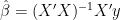
Computing directly like this in R would be
beta = solve(t(X) %*% X) %*% (X %*% y)
while in MATLAB it would be
beta = inv(X' * X) * (X' * y)

This format is handy for deriving properties of OLS analytically. But, as John says, it’s often not the best way to compute . Instead, rewrite this equation as and then get your software to solve for .
In R, this would be
beta = solve(t(X) %*% X, t(X) %*% y)
or in MATLAB, it would be
beta = (X' * X) \ (X' * y)

(Occasionally, we do actually care about the values inside an inverted matrix. Analytically we can show that, in OLS, the variance-covariance matrix of the regression coefficients is . If you really need to report these variances and covariances, I suppose you really will have to invert the matrix. But even here, if you only need them temporarily as input to something else, you can probably compute that “something else” directly without matrix inversion.)

Numerical example of problems with matrix inversion

The MATLAB documentation for inv has a nice example comparing computation times and accuracies for the two approaches.

Reddit commenter five9a2 gives an even simpler example in Octave (also works in MATLAB).

Here, I’ll demonstrate five9a2’s example in R. We’ll use their same notation of solving the system (rather than the regression example’s notation). We’ll let A be a 7×7 Hilbert matrix. The Hilbert matrices, with elements , are known to be poorly conditioned [1] and therefore to cause trouble with matrix inversion.

Here’s the R code and results, with errors and residuals defined as in the MATLAB example:

set.seed(13052015)
options(digits = 3)
library(Matrix)
library(matrixcalc)

# Set up a linear system Ax=b,
# and compare 
# inverting A to compute x=inv(A)b
# vs
# solving Ax=b directly

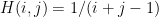
# Generate the 7x7 Hilbert matrix
# (known to be poorly conditioned)
n = 7
(A = as.matrix(Hilbert(n)))
##       [,1]  [,2]  [,3]  [,4]   [,5]   [,6]   [,7]
## [1,] 1.000 0.500 0.333 0.250 0.2000 0.1667 0.1429
## [2,] 0.500 0.333 0.250 0.200 0.1667 0.1429 0.1250
## [3,] 0.333 0.250 0.200 0.167 0.1429 0.1250 0.1111
## [4,] 0.250 0.200 0.167 0.143 0.1250 0.1111 0.1000
## [5,] 0.200 0.167 0.143 0.125 0.1111 0.1000 0.0909
## [6,] 0.167 0.143 0.125 0.111 0.1000 0.0909 0.0833
## [7,] 0.143 0.125 0.111 0.100 0.0909 0.0833 0.0769
# Generate a random x vector from N(0,1)
x = rnorm(n)
# Find the corresponding b
b = A %*% x

# Now solve for x, both ways,
# and compare computation times
system.time({xhat_inverting = solve(A) %*% b})
##    user  system elapsed 
##   0.002   0.002   0.032
system.time({xhat_solving = solve(A, b)})
##    user  system elapsed 
##   0.001   0.000   0.001

# Compare errors: sum of squared (x - xhat)
(err_inverting = norm(x - xhat_inverting))
## [1] 2.44e-07
(err_solving = norm(x - xhat_solving))
## [1] 1.56e-08

# Compare residuals: sum of squared (b - bhat)
(res_inverting = norm(b - A %*% xhat_inverting))
## [1] 1.55e-08
(res_solving = norm(b - A %*% xhat_solving))
## [1] 2.22e-16

As you can see, even with a small Hilbert matrix:

• inverting takes more time than solving;
• the error in x when solving Ax=b directly is a little smaller than when inverting; and
• the residuals in the estimate of b when solving directly are many orders of magnitude smaller than when inverting.

Repeated reuse of QR or LU factorization in R

Finally: what if, as John suggests, you have to solve Ax=b for many different b’s? How do you encode this in R without inverting A?

I don’t know the best, canonical way to do this in R. However, here are two approaches worth trying: the QR decomposition and the LU decomposition. These are two ways to decompose the matrix A into factors with which it should be easier to solve . (There are other decompositions too—many more than I want to go into here.)

QR decomposition is included in base R. You use the function qr once to create a decomposition, store the Q and R matrices with qr.Q and qr.R, then use a combination of backsolve and matrix multiplication to solve for x repeatedly using new b’s. (Q is chosen to be orthogonal, so we know its inverse is just its transpose. This avoids the usual problems with matrix inversion.)

For the LU decomposition, we can use the matrixcalc package. (Thanks to sample code on the Cartesian Faith blog.)
Imagine rewriting our problem as 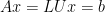, then defining , so that we can solve it in two stages: . We can collapse this in R into a single line, in the form
x = backsolve(U, forwardsolve(L, b))
once we have decomposed A into L and U.

# What if we need to solve Ax=b for many different b's?
# Compute the A=QR or A=LU decomposition once,
# then reuse it with different b's.

# Just once, on the same b as above:

# QR, Ryan's suggestion:
system.time({
  qr_decomp = qr(A, tol = 1e-10)
  qr_R = qr.R(qr_decomp)
  qr_Qt = t(qr.Q(qr_decomp))
  xhat_qr = backsolve(qr_R, qr_Qt %*% b)
})
##    user  system elapsed 
##   0.013   0.000   0.014
(err_qr = norm(x - xhat_qr))
## [1] 5.78e-08
(res_qr = norm(b - A %*% xhat_qr))
## [1] 9.44e-16

# LU, Nicholas' suggestion:
system.time({
  lu_decomp = lu.decomposition(A)
  xhat_lu = backsolve(lu_decomp$U,
                      forwardsolve(lu_decomp$L, b))
})
##    user  system elapsed 
##   0.003   0.000   0.016
(err_lu = norm(x - xhat_lu))
## [1] 3.01e-08
(res_lu = norm(b - A %*% xhat_lu))
## [1] 3.33e-16

Both the QR and LU decompositions’ errors and residuals are comparable to the use of solve earlier in this post, and much smaller than inverting A directly.

However, what about the timing? Let’s create many new b vectors and time each approach: QR, LU, direct solving from scratch (without factorizing A), and inverting A:

# Reusing decompositions with many new b's:
m = 1000
xs = replicate(m, rnorm(n))
bs = apply(xs, 2, function(xi) A %*% xi)

# QR, Ryan's suggestion:
system.time({
  qr_decomp = qr(A, tol = 1e-10)
  qr_R = qr.R(qr_decomp)
  qr_Qt = t(qr.Q(qr_decomp))
  xhats_qr = apply(bs, 2,
                   function(bi) backsolve(qr_R,
                                          qr_Qt %*% bi))
})
##    user  system elapsed 
##   0.036   0.000   0.036

# LU, Nicholas' suggestion:
system.time({
  lu_decomp = lu.decomposition(A)
  bs = apply(bs, 2,
    function(bi) backsolve(lu_decomp$U,
                           forwardsolve(lu_decomp$L, bi)))
})
##    user  system elapsed 
##   0.094   0.001   0.095

# Compare to repeated use of solve()
system.time({
  xhats_solving = apply(bs, 2,
                        function(bi) solve(A, bi))
})
##    user  system elapsed 
##   0.082   0.000   0.082

# Compare to inverting A directly
system.time({
  Ainv = solve(A)
  xhats_inverting = apply(bs, 2,
                          function(bi) Ainv %*% bi)
})
##    user  system elapsed 
##    0.01    0.00    0.01

It’s not surprising that inverting A is the fastest… but as we saw above, it’s also the least accurate, by far. Luckily, a well-done QR is almost as fast, and far more accurate.

However, I’m surprised that QR and LU are both much LU is a little slower than direct use of solve(A, b). They are LU is supposed to save you work that solve(A, b) has to redo for every new b.

Please comment if you know why this happened! Did I make a mistake? Or does LU and QR give you speedups over solve(A, b) only for much larger A matrices?

[Edit: Nicholas’ comment below and an email from Ryan Tibshirani show how to speed up the QR and LU approaches considerably. Even so, both are LU is still slower than using solve directly. See [2] for the earlier (slower) QR and LU code and results.]

[Manual pingback: Gregory Gundersen, “Why Shouldn’t I Invert That Matrix?” and a related StackExchange question.]

Finally, see this Revolutions post on R and Linear Algebra for more on matrix manipulation in R. They mention dealing with giant and/or sparse matrices, which is also the last situation described in John Cook’s blog post.

[1] (I usually hear of a “poorly conditioned” matrix, meaning one with a high “condition number,” being defined in terms of the ratio of largest to smallest eigenvalues. However, this nice supplement on Condition Numbers from Lay’s Linear Algebra has a more general definition on p.4: if A is invertible, the condition number is the norm of A times the norm of A’s inverse. This is the same as the ratio of largest to smallest eigenvalues if you’re using the spectral norm… but the general definition is more interpretable for beginners who haven’t studied eigenvalues yet, since you can use other simpler matrix norms instead.)

[2] (Here are my original approaches to QR and LU in R, using solve instead of the special cases forwardsolve and backsolve.)

# OLD VERSIONS OF QR AND LU
# (before using Nicholas's suggested improvements)

# For a single b:

# QR, first attempt:
system.time({
  qr_decomp = qr(A, tol = 1e-10)
  xhat_qr = qr.coef(qr_decomp, b)
})
##    user  system elapsed 
##   0.004   0.000   0.003
(err_qr = norm(x - xhat_qr))
## [1] 4.18e-08
(res_qr = norm(b - A %*% xhat_qr))
## [1] 6.11e-16

# QR, Nicholas' suggestion:
system.time({
  qr_decomp = qr(A, tol = 1e-10)
  R = qr.R(qr_decomp)
  xhat_qr = backsolve(R, qr.qty(qr_decomp, b))
})
##    user  system elapsed 
##   0.009   0.000   0.023
(err_qr = norm(x - xhat_qr))
## [1] 4.18e-08
(res_qr = norm(b - A %*% xhat_qr))
## [1] 6.11e-16

# LU, first attempt:
system.time({
  lu_decomp = lu.decomposition(A)
  xhat_lu = solve(lu_decomp$U, solve(lu_decomp$L, b))
})
##    user  system elapsed 
##   0.002   0.000   0.003
(err_lu = norm(x - xhat_lu))
## [1] 3.99e-08
(res_lu = norm(b - A %*% xhat_lu))
## [1] 1.11e-16

# For many b's:

# QR, first attempt:
system.time({
  qr_decomp = qr(A, tol = 1e-10)
  xhats_qr = apply(bs, 2,
                   function(bi) qr.coef(qr_decomp, bi))
})
##    user  system elapsed 
##   0.179   0.002   0.182

# QR, Nicholas' suggestion:
system.time({
  qr_decomp = qr(A, tol = 1e-10)
  qr_R = qr.R(qr_decomp)
  xhats_qr = apply(bs, 2,
    function(bi) backsolve(qr_R, qr.qty(qr_decomp, bi)))
})
##    user  system elapsed 
##   0.157   0.000   0.159

# LU, first attempt:
system.time({
  lu_decomp = lu.decomposition(A)
  bs = apply(bs, 2,
             function(bi) solve(lu_decomp$U,
                                solve(lu_decomp$L, bi)))
})
##    user  system elapsed 
##   0.167   0.001   0.173