Evil Queen of Numbers

Would there be any demand for a statistics class taught by M from the James Bond films?

M: You don’t like me, Bond. You don’t like my methods. You think I’m an accountant, a bean counter, more interested in my numbers than your instincts.
JB: The thought had occurred to me.
[…]
M: I’ve no compunction about sending you to your death, but I won’t do it on a whim.

Continue reading “Evil Queen of Numbers”

Hypothesis tests will not answer your question

Assume your hypothesis test concerns whether a certain effect or parameter is 0. With interval estimation, you can distinguish several options:

  1. The effect is precisely-measured and the interval includes 0, so we can ignore it.
  2. The effect is precisely-measured but the interval doesn’t include 0, but it’s close enough to be negligible for practical purposes, so we can ignore it.
  3. The effect is precisely-measured to be far from 0, so we can keep it as is.
  4. The effect is poorly-measured but we’re confident it’s not 0, so we can keep it but should still get more data to raise precision.
  5. The effect is poorly-measured and might be 0, so we definitely need more data before deciding what to do.

…as illustrated below:

NHST

Imagine you’re a scientist, making inferences about how the world works; or an engineer, building a tool that relies on knowing the size of these effects. You would like to distinguish between (1&2) vs. (3) vs. (4&5). Journal readers would like you to publish results for cases (1&2) or (3), and should want you to collect more data before publishing in cases (4&5).

Instead, hypothesis testing conflates (1&5) vs. (2&3&4). That doesn’t help you much!

In particular, when you conflate (1&5) it makes for bad science, as people in practice tend to interpret “not statistically significant” as “the effect must be spurious.” Instead they should interpret it as “either the effect is spurious, or it might be practically significant but not measured well enough to know.” And even if you were aware of this, and if you did collect more data to get out of situations (1&5), a hypothesis test still wouldn’t help you distinguish (2) vs. (3) vs. (4).

Finally, this is an issue whether your hypothesis tests are Frequentist or Bayesian. As John Kruschke’s excellent book on Doing Bayesian Data Analysis points out, if you do a Bayesian model comparison of one model with a spiked prior at \theta=0 and another with some diffuse prior for \theta, “all that this model comparison tells us is which of two unbelievable models is less unbelievable. [And] that is not all we want to know, because usually we also want to know what [parameter] values are credible” (p.427).

This is in addition to all the other problems with hypothesis tests. See my notes from reading Michael Oakes’ Statistical Inference for several more.

Sure, traditional hypothesis testing does have its uses, but they are rather limited. I find that interval estimation does a better job of supporting careful thought about your analysis.

audiolyzR: Data sonification with R

Update (5/15/2014): I just realized audiolyzR is publicly available on CRAN. See also co-creator Jesse Garrison’s audiolyzR page.

In his talk “Give Your Data A Listen” at last summer’s useR! 2012 conference, Eric Stone presented joint work with Jesse Garrison on audiolyzR, an R package for “data sonification.” I thought this was a nifty and well-executed idea. Since I haven’t seen Eric and Jesse post any demos online yet, I’d like to share a summary and video clip here, so that I can point to them whenever I describe audiolyzR to other folks.

audiolyzR

In August I invited Eric to my workplace to speak, and he gave us a great talk including demos of features added since the useR session. Here’s the post-event summary:

Eric Stone, a PhD student at Temple University, presented his co-authored work with Jesse Garisson on “data sonification”: using sound (other than speech) to visualize a dataset.
Eric demonstrated audiolizations of scatterplots and histograms using the statistical software R and the audio toolkit Max/MSP, as well as his ongoing research on time-series line plots. The software shows a visual display of the data and then plays an audio version, with the x-axis mapped to time and the y-axis to pitch. For instance, a positively-correlated scatterplot sounds like rising scales or arpeggios. Other variables are represented by timbre, volume, etc. to distinguish them. The analyst can also tweak the tempo and other settings while listening to the data repeatedly to help outliers stand out more clearly. A few training examples helped the audience to learn how to listen to these audiolizations and identify these outliers.
Eric believes that, even if the audiolization itself is no clearer than a visual plot, activating multiple cortices in the brain makes the analyst more attuned to the data. As a musician since childhood, he succeeded in making the results sound pleasant so that they do not wear out the listener.
The software will soon be released as an R package and linked to RExcel to expand its reach to Excel users. Future work includes: 1) supporting more data structures and more layers of data in the same audiolization; 2) testing the software with visually impaired users as a tool for accessibility; and 3) developing ways to embed the audiolizations into a website.

Eric suggested that he can imagine someone using this as part of an information dashboard or for reviewing a zillion different data views in a row, while multi-tasking: Just set it to loop through each slice of the data while you work on something else. Your ears will alert you when you hit a data slice that’s unusual and worth investigating further.

Eric has kindly sent me a version of the package, and below I demonstrate a few examples using NHANES data:

I’ve asked Eric if there’s a public release coming anytime soon, but it may be a while:

I am nearly ready to release it, but it’s one of those situations where my advisor will come up with “just one more thing” to add, so, you know, it might be a while.. Anyway, if people are interested I can provide them with the software and everything. Just let me know if anyone is.

If you want to get in touch with Eric, his contact info is in the useR talk abstract linked at the top.

On a very-loosely-related note, consider also John Cook’s post on measuring evidence in decibels. Someday I’d like to re-read this after I’ve had my morning coffee and think about if there’s any useful way to turn this metaphor into literal sonic hypothesis testing.

DC R Meetup: “Analyze US Government Survey Data with R”

I really enjoyed tonight’s DC R Meetup, presented by the prolific Anthony Damico. [Edit: adding link to the full video of Anthony’s talk; review is below.]

DamicoFlowchart (small)

I’ve met Anthony before to discuss whether the Census Bureau could either…

  • publish R-readable input statements for flat file public datasets (instead of only the SAS input statements we publish now); or…
  • cite his R package sascii, which automatically processes a SAS input file and reads data directly into R (no actual SAS installation required!). Folks agree sascii is an excellent tool and we’re working on the approvals to mention it on the relevant download pages.

Meanwhile, Anthony’s not just waiting around. He’s put together an awesome blog, asdfree.com (“Analyze Survey Data for Free”), where he posts complete R instructions for finding, downloading, importing, and analyzing each of several publicly-available US government survey datasets. These include, in his words, “obsessively commented” R scripts that make it easy to follow his logic and understand the analysis examples. Of course, “My syntax does not excuse you from reading the technical documentation,” but the blog posts point you to the key features of the tech docs. For each dataset on the blog, he also makes sure to replicate a set of official estimates from that survey, so you can be confident that R is producing the same results that it should. Continue reading “DC R Meetup: “Analyze US Government Survey Data with R””

More names for statistics, and do they matter?

Partly continuing on from my previous post

So I think we’d all agree that applied mathematics is a venerable field of its own. But are you tired of hearing statistics distinguished from “data science“? Trying to figure out the boundaries between data science, statistics, and machine learning? What skills are needed by the people in this field (these fields?), do they also need domain expertise, and are there too many posers?

Or are you now confused about what is statistics in the first place? (Excellent article by Brown and Kass, with excellent discussion and rejoinder — deserving of its own blog post soon!)

Or perhaps you are psyched for the growth of even more of these similar-sounding fields? I’ve recently started hearing people proclaim themselves experts in info-metrics and uncertainty quantification. [Edit: here’s yet another one: cognitive informatics.]

Is there a benefit to having so many names and traditions for what should, essentially, be the same thing, if it hadn’t been historically rediscovered independently in different fields? Is it just a matter of branding, or do you think all of these really are distinct specialties?

TwoTypesOfPeople

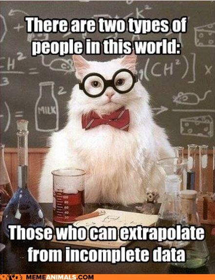
Given the position in my last post, I might argue that you should complete Chemistry Cat’s sentence with “…and those who can quantify their uncertainty about those extrapolations.” And maybe some fields have more sophisticated traditions for tackling the first part, but statisticians are especially focused on the second.

In other words, much of a statistician’s special unique contribution (what we think about more than might an applied mathematician, data scientist, haruspicer, etc.) is our focus on the uncertainty-related properties of our estimators. We are the first to ask: what’s your estimator’s bias and variance? Is it robust to data that doesn’t meet your assumptions? If your data were sampled again from scratch, or if you ran your experiment again, what’s the range of answers you’d expect to see? These questions are front and center in statistical training, whereas in, say, the Stanford machine learning class handouts, they often come in at the end as an afterthought.

So my impression is that other fields are at higher risk of modeling just the mean and stopping there (not also telling you what range of data you may see outside the mean), or overfitting to the training data and stopping there (not telling you how much your mean-predictions rely on what you saw in this particular dataset). On the other hand, perhaps traditional stats models for the mean/average/typical trend are less sophisticated than those in other communities. When statisticians limit our education to the kind of models where it’s easy to derive MSEs and compare them analytically, we miss out on the chance to contribute to the development & improvement of many other interesting approaches.

So: if you call yourself a statistician, don’t hesitate to talk with people who have a different title on their business cards, and see if your special view on the world can contribute to their work. And if you’re one of these others, don’t forget to put on your statistician hat once in a while and think deeply about the variability in the data or in your methods’ performance.

PS — I don’t mean to be adversarial here. Of course a good statistician, a good applied mathematician, a good data scientist, and presumably even a good infometrician(?) ought to have much of the same skillset and worldview. But given that people can be trained in different departments, I’m just hoping to articulate what might be gained or lost by studying Statistics rather than the other fields.

One difference between Statistics vs. Applied Math

I’ll admit it: before grad school I wasn’t fully clear on the distinction between statistics and applied mathematics. In fact — gasp! — I may have thought statistics was a branch of mathematics, rather than its own discipline. (On the contrary: see Cobb & Moore (1997) on “Mathematics, Statistics, and Teaching”William Briggs’s blog; and many others.)

Of course the two fields overlap considerably; but clearly a degree in one area will not emphasize exactly the same concepts as a degree in the other. One such difference I’ve seen is that statisticians have a greater focus on variability. That includes not just quantifying the usual uncertainty in your estimates, but also modeling the variability in the underlying population.

In many introductory applied-math courses and textbooks I’ve seen, the goal of modeling is usually to get the equivalent of a point estimate: the system’s behavior after converging to a steady state, the maximum or minimum necessary amount of something, etc. You may eventually get around to modeling the variability in the system too, but it’s not hammered into you from the start like it is in a statistics class.

For example, I was struck by some comments on John Cook’s post about (intellectual) traffic jams. Skipping the “intellectual” part for now, here’s what Cook said: Continue reading “One difference between Statistics vs. Applied Math”

Statistical Inference, Michael Oakes; and “Likelihood inference”

You may be familiar with the long-running divide between Classical or Frequentist (a.k.a. Neyman-Pearson) and Bayesian statisticians. (If not, here’s a simplistic overview.) The schism is being smoothed over, and many statisticians I know are pragmatists who feel free to use either approach depending on the problem at hand.

However, when I read Gerard van Belle’s Statistical Rules of Thumb, I was surprised by his brief mention of three distinct schools of inference: Neyman-Pearson, Bayesian, and Likelihood. I hadn’t heard of the third, so I followed van Belle’s reference to Michael Oakes’ book Statistical Inference: A Commentary for the Social and Behavioural Sciences.

Why should you care what school of inference you use? Well, it’s a framework that guides how you think about science: this includes the methods you choose to use and, crucially, how you interpret your results. Many Frequentist methods have a Bayesian analogue that will give the same numerical result on any given dataset, but the implications you can draw are quite different. Frequentism is the version taught traditionally in Stat101, but if you show someone the results of your data analysis, most people’s interpretation will be closer to the Bayesian interpretation than the Frequentist. So I was curious how “Likelihood inference” compares to these other two.

Below I summarize what I learned from Oakes about Likelihood inference. I close with some good points from the rest of Oakes’ book, which is largely about the misuse of null hypothesis significance testing (NHST) and a suggestion to publish effect size estimates instead.

Continue reading Statistical Inference, Michael Oakes; and “Likelihood inference””