
Last week I gave a short talk at CMU’s statistical computing seminar, Stat Bytes. I summarized why reproducible research (RR) and literate programming are worthwhile, not just for serious research but also for homework reports or statistical blog posts. I demonstrated how to get started with a range of RR document formats in R: from the “training wheels” R Notebook in RStudio, through the more flexible but still simple R Markdown format, to R Sweave for 
If you’ve wanted to get on the RR bandwagon, but found Sweave too overwhelming, these other tools are a great way to start—and useful in their own right, not just for training.
My materials are here:
- Overview and links (html output, Rmd source)
- R Notebook example (html output, R source)
- R Markdown example (html output, Rmd source)
- R Sweave / Beamer example (pdf output, Rnw source)
Extra details below.
Reproducible research story time
First, story time! I was once asked to step in and take over the statistical analysis for an article, after the primary statistician became unavailable. It sounded like a pretty straightforward analysis of survey data, with clear scientific questions, and they told me they had the previous statistician’s R code, so I thought it sounded reasonable. Hah…
- Not all of the variables were created in the R code: some had been created by editing columns in an Excel spreadsheet containing the data. Some of the intermediate edited columns had been deleted from the spreadsheet, so I could only guess what was done to create the final columns that I needed to use (for the sake of consistency with their prior work).
- The R code was a 50-page Word document into which they’d cut-and-pasted the R console contents. Everything they’d done, including typos and dead ends, was there for me to weed through. Well, almost everything—they must have missed copying a few critical lines of code, since I couldn’t reproduce part of their earlier results.
- The clear scientific questions turned out to be just a small subset of their questions of interest. Every time I thought I’d finished the analysis, the authors made a request to see results for another subgroup, or by another variable, or using an alternate definition of some category… For some of these requests, I couldn’t just tack on more code to the end of my script—I’d have to edit early pieces, rerun the whole thing, and email the updated results to the authors.
I’m glad I worked on this project, but it was tough to get started. In the end, I took the reproducible research approach and rewrote the analysis code as a thoroughly-documented R script that I could run from beginning to end. It was much easier to read for anyone else (or my future self) who might ever need to re-read it. And it was very simple to change a variable’s definition at the start, re-run the whole script, and have it output the tables, figures, etc. into files automatically (instead of having me copy-and-paste them from the console).
In short: even though the data are confidential and nobody’s likely to rerun my code, the reproducible research approach was critical to keeping my own work organized and manageable.
Reproducible “research” in homeworks
I also had plenty of frustrating moments last semester when grading students in a statistical computing course. Even though students wrote better R code as the semester went by, the way they wrote and reported it was not ideal. Many students wrote their homework code in the R console, then copy-and-pasted results into a text file. This way they often included mistakes in the copied code, or pasted in a result without the code that generated it.
Again, a reproducible research approach would be much easier to grade: a single R script file containing all the working code and only the working code (and comments for documentation), generating a file with all the output.
Doing reproducible research with R
So, how would you actually manage your work this way in practice? A good start is to always write your code in a script, not in the console… But how do you get away from copy-and-pasting the results into your documents (whether they’re homework, journal articles, business reports, etc.)?
The Sweave R package, designed just for this, has been around for over a decade but hasn’t gained as much traction as it should. Sweave requires learning
Recently, I’ve started (and thoroughly enjoyed) using a couple of simpler tools for this same purpose: Yihui Xie’s knitr package and RStudio. You can use knitr in regular R, without RStudio, but RStudio integrates knitr really well and adds a few features of its own. The folks at RStudio also host RPubs, a site for sharing the reports you generate with these tools. It’s very handy for homeworks (for example, see my regression homework from last term).
You can also make webpages, such as online R tutorials that intersperse regular text, R code, output, and graphics. Several good examples of knitr in use online:
- Barry Rowlingson’s tutorial on Geospatial Data in R
- Guy Lebanon’s textbook The Analysis of Data
- Rewrites in R of the data analysis examples from The Statistical Sleuth (2nd and 3rd editions)
The quickest way to get started is with RStudio’s R Notebook. Just write an R Script, then click the “Compile an HTML notebook…” button (top right corner of your script).
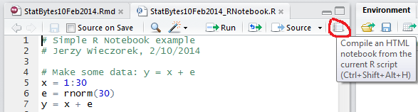
It will spit out an HTML file containing your comments and code, along with any R output and graphs. Simple and nifty. You can also do it without RStudio, using the stitch function.
Check out my R Notebook example (html output, R source) to see what I mean.
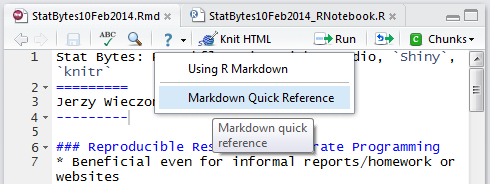
If you want to have a bit more control over the output, try R Markdown instead. Markdown itself is a document format that’s very similar to how you might write in a plain-text file: a line of dashes under a word indicates a section heading, asterisks indicate *emphasis*, etc. This gives you control over the format of your document, without having to know HTML yourself. If you create or open a RMarkdown file in RStudio, you can click the “Markdown Quick Reference” button to get a nice Markdown cheat sheet.
Then, R Markdown lets you write paragraphs of Markdown text mixed with chunks of R code and output. You use a special set of characters to indicate which chunks should be treated as R code, and the rest as Markdown text. This way (unlike in the R Notebook), you can intersperse your R code, output, and graphics with regular or formatted text and even
Here’s the R Markdown example I gave (html output, Rmd source)
One more helpful difference between R Markdown, vs. cut-and-paste from the console, is that you can paste the R Markdown output back into R easily. The results are commented out, and the commands are not:
summary(lm(y ~ x))$coefficients
##             Estimate Std. Error t value  Pr(>|t|)
## (Intercept)  -0.4657    0.37600  -1.239 2.258e-01
## x             1.0054    0.02118  47.468 2.648e-28
Whereas if you cut-and-paste from the console, you’ll get command prompts “>” as well as output results that you’d have to delete before rerunning the code:
> summary(lm(y ~ x))$coefficients
            Estimate Std. Error t value  Pr(>|t|)
(Intercept)  -0.4657    0.37600  -1.239 2.258e-01
x             1.0054    0.02118  47.468 2.648e-28
Despite R Markdown’s flexibility, the resulting HTML (though it looks great in the browser) doesn’t always print nicely, and you may need even finer control. If you are already comfortable with Sweave package or through knitr (and RStudio supports both). This is particularly useful if you need to prepare a nice academic article, or a Beamer slideshow, or a textbook. The conventions are different than in R Markdown, but knitr provides a unified framework for these documents (and keeps the code chunk options consistent). I won’t go into detail here but I included a simple Sweave + Beamer example (pdf output, Rnw source).
For more examples, documentation, etc. on all of these formats, there’s a lot of help on knitr author Yihui Xie’s website. I also want to recommend Xie’s book on Dynamic Documents with R and knitr, which starts with one of my favorite acknowledgements sections ever:
First, I want to thank my wireless router, which was broken when I started writing the core chapters of this book (in the boring winter of Ames). Besides, I also thank my wife for not giving me the Ethernet cable during that period.
Xie writes clearly and with tongue-in-cheek humor. The book is well worth reading to get a solid overview of knitr‘s potential. Yes, there is plenty of good material about knitr online already. But as Xie has said, he’s read thousands of blog-post comments and StackOverflow questions about knitr so that you don’t have to. Xie’s book also includes a list of similar tools for other languages (e.g. Python), in case this helps you convince your colleagues to get on the bandwagon. His list of reproducible research “best practices” is worth reading too. In short:
- Use relative, not absolute, file paths and keep a whole project in one directory whenever possible
- Don’t change the working directory—maybe OK at the very start of your script, but not later
- Compile your reports in a clean R session to make sure they’re not “contaminated” by existing R objects
- Avoid any commands needing human interaction, and avoid relying on environment variables outside the code; the whole script should be automated and self-contained
- Include the sessionInfo() and instructions on running/compiling the document for your collaborators (or future self)
One weird NEW trick
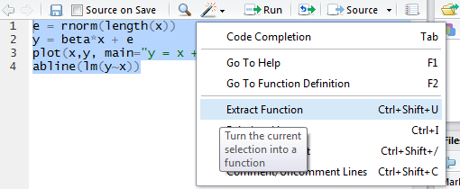
One last RStudio tip: if you write a block of R code, then realize you wish you’d written it as a function instead… They have a command for this, called “Extract Function”:
RStudio can analyze a selection of code from within the source editor and automatically convert it into a re-usable function. Any “free” variables within the selection (objects that are referenced but not created within the selection) are converted into function arguments.
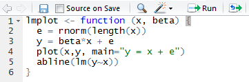
Before:
And after:
Thanks, Jerzy, for all the kind words! I do not care what you said about RR, but I’m really glad that you found the acknowledgements amusing. Just kidding 🙂
Along other productivity methods like GTD or Pomodoro, you should start marketing your own method: SRI = Spouse Removes Internet. It works for me too 🙂