`surveyCV`: K-fold cross validation for complex sample survey designs

I’m fortunate to be able to report the publication of a paper and associated R package co-authored with two of my undergraduate students (now alums), Cole Guerin and Thomas McMahon: “K-Fold Cross-Validation for Complex Sample Surveys” (2022), Stat, doi:10.1002/sta4.454 and the surveyCV R package (CRAN, GitHub).

The paper’s abstract:

Although K-fold cross-validation (CV) is widely used for model evaluation and selection, there has been limited understanding of how to perform CV for non-iid data, including from sampling designs with unequal selection probabilities. We introduce CV methodology that is appropriate for design-based inference from complex survey sampling designs. For such data, we claim that we will tend to make better inferences when we choose the folds and compute the test errors in ways that account for the survey design features such as stratification and clustering. Our mathematical arguments are supported with simulations and our methods are illustrated on real survey data.

Long story short, traditional K-fold CV assumes that your rows of data are exchangeable, such as iid draws or simple random samples (SRS). But in survey sampling, we often use non-exchangeable sampling designs such as stratified sampling and/or cluster sampling.¹

Illustration of simple random sampling, stratified sampling, and cluster sampling

Our paper explains why in such situations it can be important to carry out CV that mimics the sampling design.² First, if you create CV folds that follow the same sampling process, then you’ll be more honest with yourself about how much precision there is in the data. Next, if on these folds you train fitted models and calculate test errors in ways that account for the sampling design (including sampling weights³), then you’ll generalize from the sample to the population more appropriately.

If you’d like to try this yourself, please consider using our R package surveyCV. For linear or logistic regression models, our function cv.svy() will carry out the whole K-fold Survey CV process:

generate folds that respect the sampling design,
train models that account for the sampling design, and
calculate test error estimates and their SE estimates that also account for the sampling design.

For more general models, our function folds.svy() will partition your dataset into K folds that respect any stratification and clustering in the sampling design. Then you can use these folds in your own custom CV loop. In our package README and the intro vignette, we illustrate how to use such folds to choose a tuning parameter for a design-consistent random forest from the rpms R package.

Finally, if you are already working with the survey R package and have created a svydesign object or a svyglm object, we have convenient wrapper functions folds.svydesign(), cv.svydesign(), and cv.svyglm() which can extract the relevant sampling design info out of these objects for you.

It was very rewarding to work with Cole and Thomas on this project. They did a lot of the heavy lifting on setting up the initial package, developing the functions, and carrying out simulations to check whether our proposed methods work the way we expect. My hat is off to them for making the paper and R package possible.

Some next steps in this work:

Find additional example datasets and give more detailed guidance around when there’s likely to be a substantial difference between usual CV and Survey CV.
Build in support for automated CV on other GLMs from the survey package beyond the linear and logistic models. Also, write more examples of how to use our R package with existing ML modeling packages that work with survey data, like those mentioned in Section 5 of Dagdoug, Goga, and Haziza (2021).
Try to integrate our R package better with existing general-purpose R packages for survey data like srvyr and for modeling like tidymodels, as suggested in this GitHub issue thread.
Work on better standard error estimates for the mean CV loss with Survey CV. For now we are taking the loss for each test case (e.g., the squared difference between prediction and true test-set value, in the case of linear regression) and using the survey package to get design-consistent estimates of the mean and SE of this across all the test cases together. This is a reasonable survey analogue to the standard practice for regular CV—but alas, that standard practice isn’t very good. Bengio and Grandvalet (2004) showed how hard it is to estimate SE well even for iid CV. Bates, Hastie, and Tibshirani (2021) have recently proposed another way to approach it for iid CV, but this has not been done for Survey CV yet.

Meng’s “Big Data Paradox” and an extreme example

Update (December 2021): Welcome, new readers. I’m seeing an uptick in visits to this post, probably due to the Nature paper that was just published: “Unrepresentative big surveys significantly overestimated US vaccine uptake” (Bradley et al., 2021). I’ve added a short post with a bit more about the Bradley paper. But the main point is that I strongly encourage you to also read Frauke Kreuter’s brief “What surveys really say,” which describes the context for all of this and points to some of the research challenges needed in order to move ahead; and Reinhart & Tibshirani’s “Big data, big problems,” the Delphi-Facebook survey team’s response to (an earlier draft of) Bradley et al. That said, I hope my 2018 post below is still a useful glimpse at the Big Data Paradox idea.

Original post (October 2018): Xiao-Li Meng’s recent article on “Statistical Paradises and Paradoxes in Big Data (I)” has a fascinating approach to quantifying uncertainty in the Big Data setting. Here’s a very loose/oversimplified summary, along with an extreme example of applying some of these ideas. But I certainly encourage you to read the original paper itself.

(Hat tip: Lee Richardson, and CMU’s History of Statistics reading group.)

We exhort our Intro Stats students: Don’t trust data from a biased sample! Yet in the real world, we rarely deal with datasets collected under a formal random sampling scheme. Sometimes we have e.g. administrative data collected from many people but only those who self-selected into the sample. Even when we do take a “proper” random survey, there is usually nonignorable non-response.

Meng tackles the question: When does a small random survey really give better estimates than a large non-random dataset? He frames the problem gracefully in a way which highlights the importance of two things: (1) the correlation between *whether* a person responds and *what* their response is, and (2) the overall population size N (not just the observed sample size n). Under simple random sampling, the correlation should be essentially 0, and the usual standard error estimates are appropriate. But when we have non-random sample selection, this correlation leads to bias in our estimates, in a way such that the bias gets *substantially worse* when the population is large and we have a large sampling fraction n/N.

Meng reframes the problem several ways, but my favorite is in terms of “effective sample size” or n_eff. For a particular n, N, and correlation, quantify the uncertainty in our estimate—then figure out what sample size from a simple random sample would give the same level of uncertainty. In an extended example around the 2016 US presidential election, Meng suggests that there was a small but non-zero correlation (around 0.005) between *whether* you responded to polling surveys and *which* candidate you supported, Trump or Clinton. This tiny correlation was enough to affect the polling results substantially. All the late election poll samples added up to about 2 million respondents, which at first seems like a massive sample size—naive confidence intervals would have tiny margins of error, less than 1/10th of a percentage point. Yet due to that small correlation of 0.005 (Trump voters were a tiny bit less likely to respond to polls than Clinton voters were), the effective sample size n_eff was around 400 instead, with a margin of error around 5 percentage points.

Let’s say that again: Final estimates for the percent of popular vote going to Trump vs Clinton were based on 2 million respondents. Yet due to self-selection bias (who agreed to reply to the polls), the estimates’ quality was no better than a simple random survey of only 400 people, if you could get a 100% response rate from those 400 folks.

On the other hand, if you want to try correcting your own dataset’s estimates and margins of error, estimating this correlation is difficult in practice. You certainly can’t do it from the sample at hand, though you can try to approximate it from several samples. Still, one rough estimate of n_eff gives some insight into how bad the problem can get.

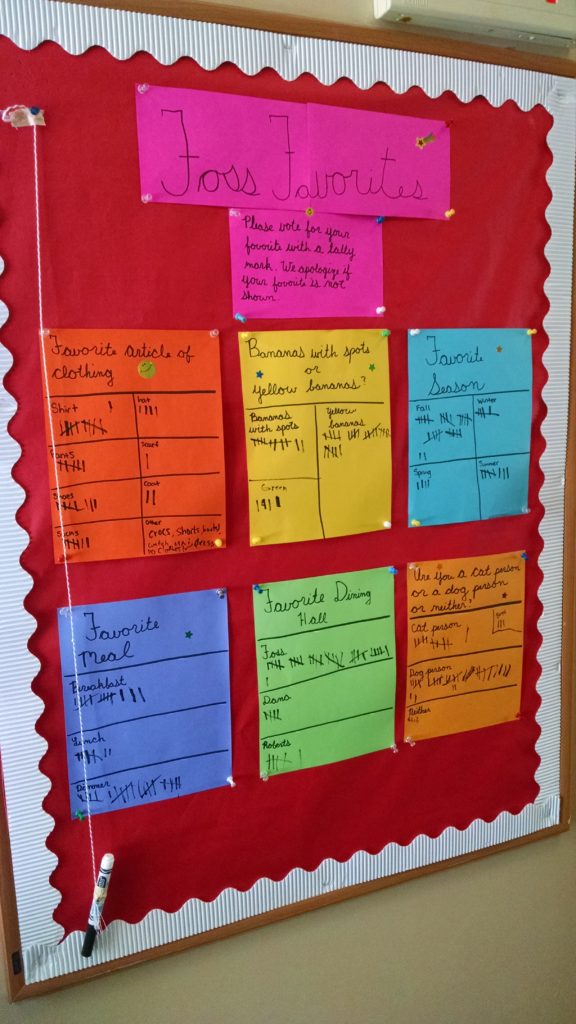
Here at Colby College, students have a choice of three dining halls: Foss, Roberts (affectionately called Bobs), and Dana. Around the start of the year, I saw this informal “survey” near the entrance to Foss:

Students walking past the bulletin board were encouraged to make a tally mark near their favorite season, favorite article of clothing, etc… and their favorite dining hall. Here, Foss is far in the lead, with 32 votes compared to 5 and 6 for Dana and Roberts respectively. But of course, since this bulletin board is at Foss, you only get passers-by who are willing to go to Foss. We talked about this in class as an example of (highly!) biased sampling.

Now, I want to go further, using one of Meng’s effective sample size estimates. Let’s say that we want to estimate the proportion of Colby students whose favorite dining hall is Foss. Meng’s equation (4.4) estimates the effective sample size as

n_eff = 4 * (n/N)^2 * (1/delta)^2

where delta is the expected difference in [probability of responding for people who prefer Foss] versus [probability of responding for people who prefer another dining hall]. The bulletin board showed about n = 43 respondents, which is roughly 1/40th of the 2000-ish student body, so let’s assume n/N = 1/40. In that case, if delta is any larger than 0.05, n_eff is estimated to be 1.

It certainly seems reasonable to believe that Prob(respond to a survey in Foss | you prefer Foss) is at least 5 percentage points higher than Prob(respond to a survey in Foss | you prefer some other dining hall). Foss is near the edge of campus, close to dorms but not classrooms. If you *don’t* prefer the food at Foss, there’s little reason to pass by the bulletin board, much less to leave a tally mark. In other words, delta = 0.05 seems reasonable… which implies that n_eff <= 1 is reasonable… which means this “survey” is about as good as asking ONE random respondent about their favorite dining hall!

[Edit: for a sanity check on delta’s order of magnitude, imagine that in fact about 1/3 of Colby’s students prefer each of the 3 dining halls. So we got around 30/600ish Foss-preferrers responding here, for around a 0.05 response rate. And we got around 12/1200ish of the other students responding here, for around a 0.01 response rate. So the difference in response rates is 0.04. That’s a bit lower than our extreme hypothesized delta = 0.05, but it is in a reasonable ballpark.]

In general, if delta is around twice n/N, we estimate n_eff = 1. Even if we waited to get a much larger sample, say 200 or 250 students leaving tally marks on the board, the survey is still useless if we believe delta >= 0.01 is plausible (which I do).

There’s plenty more of interest in Meng’s article, but this one takeaway is already enough to be fascinating for me—and a nifty in-class example for just *how* bad convenience sampling can be.

“Statistical Modeling: The Two Cultures,” Breiman

One highlight of my fall semester is going to be a statistics journal club led by CMU’s Ryan Tibshirani together with his dad Rob Tibshirani (here on sabbatical from Stanford). The journal club will focus on “Hot Ideas in Statistics“: some classic papers that aren’t covered in standard courses, and some newer papers on hot or developing areas. I’m hoping to find time to blog about several of the papers we discuss.

The first paper was Leo Breiman’s “Statistical Modeling: The Two Cultures” (2001) with discussion and rejoinder. This is a very readable, high-level paper about the culture of statistical education and practice, rather than about technical details. I strongly encourage you to read it yourself.

Breiman’s article is quite provocative, encouraging statisticians to downgrade the role of traditional mainstream statistics in favor of a more machine-learning approach. Breiman calls the two approaches “data modeling” and “algorithmic modeling”: Continue reading ““Statistical Modeling: The Two Cultures,” Breiman” →