R101

I’m preparing “R101,” an introductory workshop on the statistical software R. Perhaps other beginners might find some use in the following summary and resources. (See also the post on resources for teaching yourself introductory statistics.)

Do you have obligatory screenshots of nifty graphics that R can produce? Yes, we do.

Nice. So what exactly is R? It is an open-source software tool for statistics, data processing, data visualization, etc. (Technically there’s a programming language called S, and R is just one open-source software tool that implements the S language. But you’ll often hear people just say “the R language.” Beginners can worry about the nuances later.)
Open source means it is free to download and use; this is great for academics and others with low budgets. It also means you can inspect the code of any algorithm if you want to double-check it or just to see how it’s done; this is great for validating and building on each others’ ideas. And it is easy to share code in user-defined “packages,” of which there are thousands, all helping people use cutting-edge statistical tools as soon as they are invented.

How do I get started? Download and install R from CRAN, the Comprehensive R Archive Network. There are Windows, Mac, and Linux versions.
In Windows at least, when you open the program there is a big window containing a smaller window, the R Console. You can type and submit commands in the Console window at the prompts (the “>” signs). Try typing 3+5 and hit Enter, and you should see the output [1] 8 which is good. The output of 3+5 is a 1-item vector (hence the [1]) with the value 8 as it should be.
Great, now you know how to use R as a desktop calculator!
Or you can type your commands in a script, so that you can save your code easily. Go to “File -> New script” and it will open the R Editor window. Type 3+5 in there, highlight it, and then either click the “Run line or selection” icon on the top menu bar or just hit Ctrl+R on the keyboard. It should copy the command into the Console window and run it, with the same result as before.
Sweet, now you can save the code you used to do your calculations.
Quick-R has more details on using the R interface.
Next, try A Sample Session from the R manual to see examples of other things R can do.

What are the key concepts? Basically, everything is a function or an object. Objects are where your data and results are stored: data frames, matrices, vectors, lists, etc. Functions take objects in, think about them, and spit new objects out. Functions sometimes also have side effects (like displaying a table of output or a graph, or changing a display setting).
If you want to save the results or output of a function, use <- which is the assignment operator (think of an arrow pointing left). For example, to save the natural log of 10 into a variable called x, type the command x <- log(10). Then you can use x as the input to another function.
Note that functions create new output rather than affecting the input variable. If you have a vector called y that you need sorted, sort(y) will print out a sorted copy of y but will not changed y itself. If you actually want y to be sorted, you have to reassign it: y <- sort(y).
Functions always take their input in parentheses: (). So if you see a word followed by parentheses, you know it’s a function in R. You will also see square brackets: []. These are used for locating or extracting data in objects. For example, if you have a vector called y, then y[3] gives you the 3rd element of that vector. If y is a matrix, then y[4,7] is the element in the 4th row, 7th column.

How do I get help? If you know you want to use a function named foo, you can learn more about it by typing ?foo which will bring up the help file for that function. The “Usage” section tells you the arguments, their default order, and their default values. (If no default value is given, it is a required argument.) “Arguments” gives more details about each argument. “Value” gives the structure of the output. “Examples” shows an example of the function in use.
If you know what you want to do but don’t know what the function is called, I suggest looking through the R Reference Card. If that does not answer your question, you can try searching using RSeek.org or search.r-project.org, search engine tuned to the R sites and mailing lists… since just typing the letter R into Google is not always helpful 🙂

For statisticians used to other packages:
Quick-R
R for SAS and SPSS Users

For programmers:
R’s unconventional features
Google’s R code style guide

Good books (as suggested by Cosma Shalizi):
Paul Teetor, The R Cookbook: “explains how to use R to do many, many common tasks”
Norman Matloff, The Art of R Programming: “Good introduction to programming for complete novices using R.”

Separation of degrees

Scientific American has a short article on trends in undergraduate degrees over the past 20 years, illustrated with a great infographic by Nathan Yau. As a big fan of STEM (science, tech, engineering and math) education, I was pleased to see data on changing patterns among STEM degree earners.

However, there seemed to be a missed opportunity. The article mentioned that “More women are entering college, which in turn is changing the relative popularity of disciplines.” If the data were broken down by gender, readers could better see this fact for themselves.

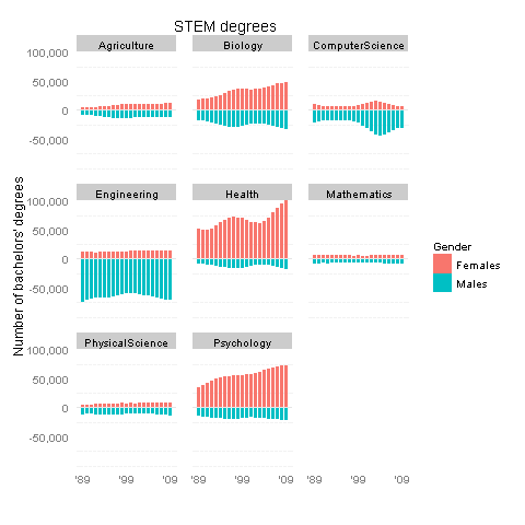
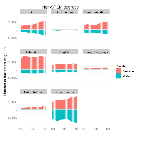
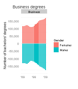
I thought I could exploit the current graphic’s slight redundancy: the bar heights below and above the gray horizontal lines are exactly the same. Why not repurpose this format to show data on degrees earned by men vs. by women (below vs. above the horizontal line), in the same amount of space?

I could not find the gender breakdown for the exact same set of degrees, but a similar dataset is in the Digest of Education Statistics, tables 308 to 330. Here are my revised plots, made using R with the ggplot2 package.

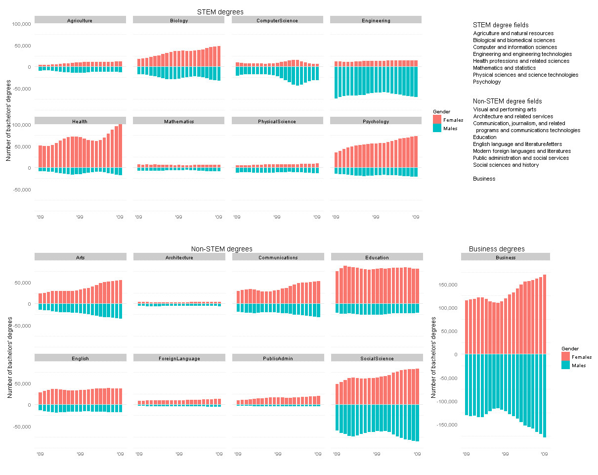
Click this thumbnail to see all the data in one plot (it’s too big for the WordPress column width):

Or see the STEM and non-STEM plots separately below.

So, what’s the verdict? These new graphs do support SciAm’s conclusions: women are largely driving the increases in psychology and biology degrees (as well as “health professions and related sciences”), and to a lesser degree in the arts and communications. On the other hand, increases in business and social science degrees appear to be driven equally by males and females. The mid-’00s spike in computer science was mostly guys, it seems.

I’d also like to think that my alma mater, Olin College, contributed to the tiny increase in female engineers in the early ’00s 🙂

Technical notes:
Some of these degree categories are hard to classify as STEM vs. non-STEM. In particular, Architecture and SocialScience include some sub-fields of each type… Really, I lumped them under non-STEM only because it balanced the number of items in each group.
Many thanks to a helpful Learning R tutorial on back-to-back bar charts.

Spinner Doctor

The setup

Dan Meyer, a (former?) math teacher with some extraordinary ideas, has a nifty concept for teaching expected values:

“So one month before our formal discussion of expected value, I’d print out this image, tack a spinner to it, and ask every student to fix a bet on one region for the entire month. I’d seal my own bet in an envelope.

I’d ask a new student to spin it every day for a month. We’d tally up the cash at the end of the month as the introduction to our discussion of expected value.
So let them have their superstition. Let them take a wild bet on $12,000. How on Earth did the math teacher know the best bet in advance?”

I absolutely love the idea of warming up their brains to this idea a month before you actually teach it, and getting them “hooked” by placing a bet and watching it play out over time.

The Challenge

But there’s a problem: at least as presented, the intended lesson isn’t quite true. I’m taking it as a challenge to see if we can fix it without killing the wow-factor. Let’s try.

As I read it, the intended lesson here is: “if you’re playing the same betting game repeatedly, it’s good to bet on the option with the highest expected value.”
And the intended wow-factor comes from: “none of the options looked like an obvious winner to me, but my teacher knew which one would win!”

But the lesson just isn’t true with this spinner and time-frame: here, the highest-expected-value choice is actually NOT the one most likely to have earned the most money after only 20 or 30 spins.
And the wow-factor is not guaranteed: none of the choices is much more likely to win than the others in only 20-30 spins, so the teacher can’t know the winning bet in advance. It’s like you’re a magician doing a card trick that only works a third of the time. You can still have a good discussion about the math, but it’s just not as cool.

I’d like to re-design the spinner so that the lesson is true, and the wow-factor still happens, after only a month of spins.

WAit, is there really a problem?

First, what’s wrong with the spinner? By my eyeball, the expected values per spin are $100/2 = $50; $300/3 = $100; $600/9 = $67ish; $5000/27 = $185ish; and $12000/54 = $222ish. So in the LONG run, if you spin this spinner a million times, the “$12000” has the highest expected value and is almost surely the best bet. No question.

But in Dan’s suspense-building setup, you only spin once a day for a month, for a total of 20ish spins (since weekends are out). With only 20 spins, the results are too unpredictable with the given spinner — none of the five choices is especially likely to be the winner.

How do we know? Instead of thinking “the action is spinning the spinner once, and we’re going to do this action twenty times,” let’s look at it another way: “the action is spinning the spinner twenty times in a row, and we’re going to do this action once.” That’s what really matters to the classroom teacher running this exercise: you get one shot to confidently place my bet at the start of the month; after a single month of daily spins, will the kids be wowed by seeing that you placed the right bet?

I ran a simulation in R (though sometime I’d like to tackle this analytically too):
Take 20 random draws from a multinomial distribution with the same probabilities as Dan’s spinner.
Multiply the results by the values of each bet.

> nr.spins <- 20
> spins=rmultinom(1,size=nr.spins,prob=c(1/2,1/3,1/9,1/27,1/54))
> spins
     [,1]
[1,]   11
[2,]    7
[3,]    2
[4,]    0
[5,]    0
> winnings=spins*c(100,300,600,5000,12000)
> winnings
     [,1]
[1,] 1100
[2,] 2100
[3,] 1200
[4,]    0
[5,]    0

For example, in this case we happened not to hit the “$5000” or the “$12000” at all. But we hit “$100” 11 times, “$300” 7 times, and “$600” twice, so someone who bet on “$300” would have won the most money that month.
Now, this was just for one month. Try it again for another month:

> spins
     [,1]
[1,]    8
[2,]    9
[3,]    1
[4,]    2
[5,]    0
> winnings
      [,1]
[1,]   800
[2,]  2700
[3,]   600
[4,] 10000
[5,]     0

This time we got “$5000” twice and whoever bet on that would have been the winner.
Okay, there’s clearly some variability as to who wins when you draw a new set of 20 spins. We want to know how variable this is.
So let’s do this many times — like a million times — and each time you do it, see which bet won that month. Keep track of how often each bet wins (and ties too, why not).

nr.sims=1000000
bestpick <- rep(0,5)
tiedpick <- rep(0,5)
nr.spins <- 20
for(i in 1:nr.sims){
    spins=rmultinom(1,size=nr.spins,prob=c(1/2,1/3,1/9,1/27,1/54))
    winnings=spins*c(100,300,600,5000,12000)
    best <- which(winnings==max(winnings))
    if(length(best)==1){
        bestpick[best] <- bestpick[best]+1
    } else{
        tiedpick[best] <- tiedpick[best]+1
    }
}

Results are as follows. The first number under bestpick is the rough proportion of times that “$100” would win; the last number is the rough proportion of times that “$12000” would win. Similarly for proportion of ties under tiedpick, except that I haven’t corrected for double-counting (since ties are rare enough not to affect our conclusions).

> bestpick/nr.sims
[1] 0.0145 0.2124 0.0712 0.3780 0.3029
> tiedpick/nr.sims
[1] 0.00199 0.02093 0.01893 0.00000 0.0000

(Ties, and the fact it’s just a simulation, mean these probabilities aren’t exactly right… but they’re within a few percentage points of their long-run value.)
It turns out that the fourth choice, “$5000”, wins a little under 40% of the time. The highest-expected-value choice, “$12000”, only wins about 30% of the time. And “$300” turns out to be the winning bet about 20% of the time.
Unless I’ve made a mistake somewhere, this shows that using Dan’s spinner for one spin a day, 20 days in a row, (1) the most likely winner is not the choice with the highest expected value, and (2) the teacher can’t know which choice will be the winner — it’s too uncertain. So the lesson is wrong, and you can’t guarantee the wow-factor. That’s a shame.

dang. What to do, then?

Well, you can try spinning it more than once a day. What if you spin it 10 times a day, for a total of 200 spins? If we re-run the simulation above using nr.spins <- 200 here’s what we get:

> bestpick/nr.sims
[1] 0.000000 0.012258 0.000287 0.393095 0.589246
> tiedpick/nr.sims
[1] 0.000000 0.000332 0.000037 0.004780 0.005079

So it’s better, in that “$12000” really is the best choice… but it still has only about a 60% chance of winning. I’d prefer something closer to 90% for the sake of the wow-factor.
What if you have each kid spin it 10 times each day? Say 20 kids in the class, times 10 spins per kid, times 20 days, so 4000 spins by the month’s end:

> bestpick/nr.sims
[1] 0.000 0.000 0.000 0.106 0.892
> tiedpick/nr.sims
[1] 0.00000 0.00000 0.00000 0.00157 0.00157

That’s much better. But that’s a lot of spins to do by hand, and to keep track of…
Of course you could run a simulation on your computer, but I assume that’s nowhere near as convincing to the students.

What I’d really like to see is a spinner that gives more consistent results, so that you can be pretty sure after only 20 or 30 spins it’ll usually give the same winner. A simple example would be a spinner with only these 3 options: 1/2 chance of $100, 1/3 chance of $300, and 1/6 chance of $400.

> bestpick/nr.sims
[1] 0.0574 0.6977 0.2371
> tiedpick/nr.sims
[1] 0.00200 0.00783 0.00596

That’s okay, but there’s still only about a 70% chance of the highest-expected-value (“$300” here) being the winner after 20 spins… and anyway it’s much easier to guess “correctly” here, no math required, so it’s not as impressive if the teacher does guess right.

Hmmm. Gotta think a bit harder about whether it’s possible to construct a spinner that’s both (1) predictable and (2) non-obvious, given only 20 or so spins. Let me know if you have any thoughts.

Edit: I propose a better solution in the next post.

The Testimator: Significance Day

A few more thoughts on JSM, from the Wednesday sessions:

I enjoyed the discussion on the US Supreme Court’s ruling regarding statistical significance. Some more details of the case are here.
In short, the company Matrixx claimed they did not need to tell investors about certain safety reports, since those results did not reach statistical significance. Matrixx essentially suggested that there should be a “bright line rule” that only statistically-significant results need to be reported.
However, the Supreme Court ruled against this view: All of the discussants seemed to agree that the Supreme Court made the right call in saying that statistical significance is not irrelevant, but we have to consider “the totality of the evidence.” That’s good advice for us all, in any context!

In particular, Jay Kadane and Don Rubin did not prepare slides and simply spoke well, which was a nice change of presentation style from most other sessions. Rubin brought up the fact that the p-value is not a property solely of the data, but also of the null hypothesis, test statistics, covariate selection, etc. So even if the court wanted a bright-line rule of this sort, how could they specify one in sufficient detail?
For that matter, while wider confidence intervals are more conservative
when trying to showing superiority of one drug over another, there are safety situations where narrower confidence intervals are actually the more conservative ones but “everyone still screws it up.” And “nobody really knows how to do multiple comparisons right” for subgroup analysis to check if the drug is safe on all subgroups. So p-values are not a good substitute for human judgment on the “totality of the evidence”.

I also enjoyed Rubin’s quote from Jerzy Neyman: “You’re getting misled by thinking that the mathematics is the statistics. It’s not.” This reminded me of David Cox’s earlier comments that statistics is about the concepts, not about the math. In the next session, Paul Velleman and Dick DeVeaux continued this theme by arguing that “statistics is science more than math.”
(I also love DeVeaux and Velleman’s 2008 Amstat News article on how “math is music; statistics is literature.” Of course Andrew Gelman presented his own views about stats vs. math on Sunday; and Perci Diaconis talked about the need for conceptually-unifying theory, rather than math-ier theory, at JSM 2010. See also recent discussion at The Statistics Forum. Clearly, defining “statistics” is a common theme lately!)

In any case, Velleman presented a common popular telling of the history behind Student’s t test, and then proceeded to bust myths behind every major point in the story. Most of all, he argued that we commonly take the wrong lessons from the story. Perhaps it was not his result (the t-test) that should be taught so much as the computationally-intensive method he first used, which is an approach that’s easier to do nowadays and may be more pedagogically valuable.
I’m also jealous of Gosset’s title at Guinness: “Head Experimental Brewer” would look great on a resume 🙂

After their talks, I went to the session honoring Joe Sedransk in order to hear Rod Little and Don Malec talk about topics closer to my work projects. Little made a point about “inferential schizophrenia”: if you use direct survey estimates for large areas, and model-based estimates for small areas, your entire estimation philosophy jumps drastically at the arbitrary dividing line between “large” and “small.” Wouldn’t it be better to use a Bayesian approach that transitions smoothly, closely approaching the direct estimates for large areas and the model estimates in small areas?
Pfeffermann and Rao commented afterwards that they don’t feel things are as “schizophrenic” as Little claims, but are glad that Bayesians are now okay with measuring the frequentist properties of their procedures (and Little claimed that Bayesian models can often end up with better frequentist properties than classical models).

In the afternoon, I sat in on Hadley Wickham’s talk about starting off statistics courses with graphical analysis.This less-intimidating approach lets beginners describe patterns right from the start.
He also commented that each new tool you introduce should be motivated by an actual problem where it’s needed: find an interesting question that is answered well by the new tool. In particular, when you combine a good dataset with an interesting question that’s well-answered by graphics, this gives students a good quick payoff for learning to program. Once they’re hooked, *then* you can move to the more abstract stuff.

Wickham grades students on their curiosity (what can we discover in this data?), skepticism (are we sure we’ve found a real pattern?), and organization (can we replicate and communicate this work well?). He provides practice drills to teach “muscle memory,” as well as many opportunities for mini-analyses to teach a good “disposition.”
This teaching philosophy reminds me a lot of Dan Meyer and Shawn Cornally’s approaches to teaching math ~~(which I will post about separately sometime)~~ (edit: which I have posted about elsewhere).
Wickham also collects interesting datasets, cleans them up, and posts them on Github along with his various R packages and tools including the excellent ggplot2.

The last talks I attended (by Eric Slud and Ansu Chatterjee, on variance estimation) were also related to my work on small area modeling.
I was amused by the mixed metaphors in Chatterjee’s warning to “not use the bootstrap as a sledgehammer,” and Bob Fay’s discussion featured the excellent term “Testimator” 🙂
This reminds me that last year Fay presented on the National Crime Victimization Survey, and got a laugh from the audience for pointing out that, “From a sampling point of view, it’s a problem that crime has gone down.”

Overall, I enjoyed JSM (as always). I did miss a few things from past JSM years:
This year I did not visit the ASA Student Stat Bowl competition, and I’m a bit sad that as a non-student I can no longer compete and defend my 2nd place title… although that ranking may not have held up across repeated sampling anyway 😛
I was also sad that last year’s wonderful StatAid / Statistics Without Borders mixer could not be repeated this year due to lack of funding.
But JSM was still a great chance to meet distant friends and respected colleagues, get feedback on my research and new ideas on many topics, see what’s going on in the wider world of stats (there are textbooks on Music Data Mining now?!?), and explore another city.
(Okay, I didn’t see too much of Miami beyond Lincoln Rd,
but I loved that the bookstore was creatively named Books & Books …
and the empanadas at Charlotte Bakery were outstanding!)
I also appreciate that it was an impetus to start this blog — knock on wood that it keeps going.

I look forward to JSM 2012 in San Diego!