I’ve updated the interactive poverty map from last month, providing better labels, legends, and a clickable link to the data source. It also actually compares confidence intervals correctly now. I may have switched the orange and purple colors too. (I also reordered the code so that things are defined in the right order; I think that was why sometimes you’d need to reload the map before the interactivity would work.)

Please click the screenshot to try the interactive version (seems to work better in Firefox than Internet Explorer):

Next steps: redo the default color scheme so it shows the states relative to the national average poverty rate; figure out why there are issues in the IE browser; clean up the code and share it on Github.
[Edit: the IE issues seem to be caused by D3’s use of the SVG format for its graphics; older versions of IE do not support SVG graphics. I may try to re-do this map in another Javascript library such as Raphaël, which can apparently detect old versions of IE and use another graphics format when needed.]

For lack of a better term I’m still using “idiopleth”: idio as in idiosyncratic (i.e. what’s special about this area?) and pleth as in plethora (or choropleth, the standard map for a multitude of areas). Hence, together, idiopleth: one map containing a multitude of idiosyncratic views. Please leave a comment if you know of a better term for this concept already.

In which we propose a unifying theme, name, and some new prototypes for visualizations that allow “localization of comparisons,” aka “How do I relate to others?”

When Nathan Yau visited the Bureau a few months ago, he compared two world maps of gasoline prices by country. The first one was your typical choropleth: various color shades correspond to different gas prices. Fair enough, but (say) an American viewing the map is most likely interested in how US gas prices compare to the rest of the world. So instead, present a map with America in a neutral color (grey) and recolor the other countries relative to the US, to show whether their prices are higher or lower than here (for instance, red for pricier and green for cheaper gas).

I liked this idea but wanted to take it further: Instead of a one-off map just for Americans, why not make an interactive map that recolors automatically when you select a new country?
As a statistician, I’m also interested in how to communicate uncertainty: is your local area’s estimate statistically significantly different from your neighbors’ estimates? Continue reading “Localized Comparisons: Idiopleth Maps?” →

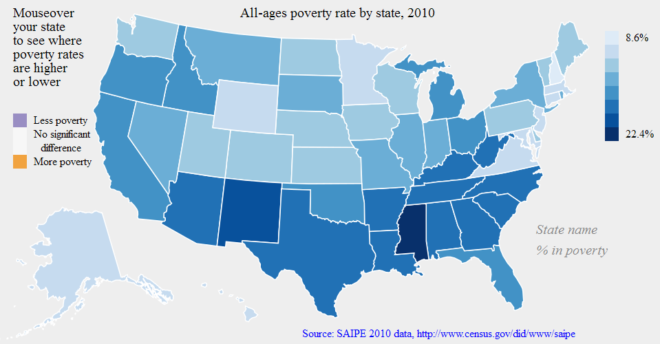
Yesterday I had the pleasure of eating lunch with Nathan Yau of FlowingData.com, who is visiting the Census Bureau this week to talk about data visualization.
He told us a little about his PhD thesis topic (monitoring, collecting, and sharing personal data). The work sounds interesting, although until recently it had been held up by work on his new book, Visualize This.

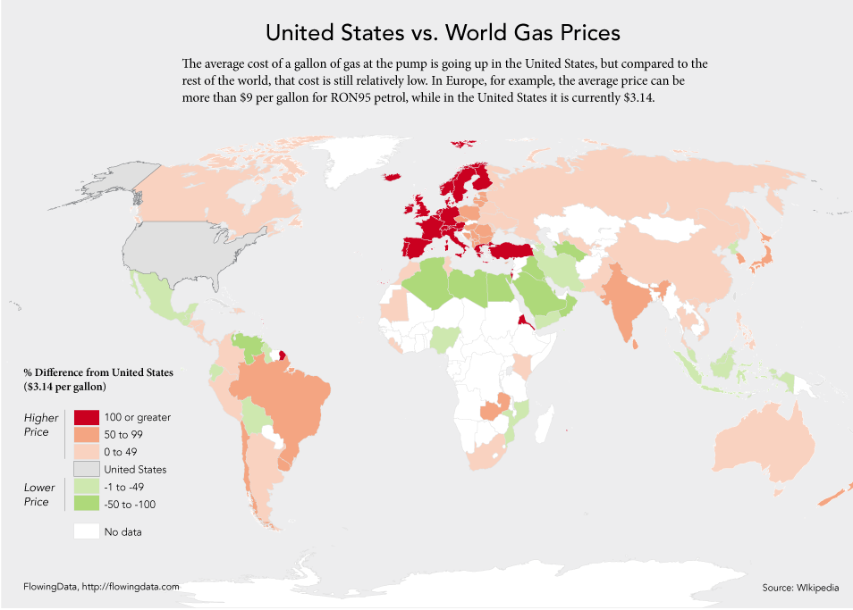
We also talked about some recent online discussions of “information visualization vs. statistical graphics.” These conversations were sparked by the latest Statistical Computing & Graphics newsletter. I highly recommend the pair of articles on this topic: Robert Kosara made some great points about the potential of info visualization, and Andrew Gelman with Antony Unwin responded with their view from the statistics side.

In Yau’s opinion, there is not much point in making a difference between the two. However, as I understand it, Gelman then continued blogging on this topic but in a way that may seem critical towards the info visualization community:
“Lots of work to convey a very simple piece of information,” “There’s nothing special about the top graph above except how it looks,” “sacrificing some information for an appealing look” …
Kaiser Fung, of the Junk Charts blog, pitched in on the statistics side as well. Kosara and Yau responded from the visualization point of view.
To all statisticians, I recommend Kosara’s article in the newsletter and Yau’s post which covers the state of infovis research.

My view is this: Gelman seems intent on pointing out the differences between graphs made by statisticians with no design expertise vs. by designers with no statistical expertise, but I don’t think this latter group represents what Kosara is talking about. Kosara wants to highlight the potential benefits for a person (or team) who can combine both sets of expertise. These are two rather different discussions, though both can contribute to the question of how to train people to be fluent in both skill-sets.

Personally, I can think of examples labeled “information visualization” that nobody would call “statistical graphics” (such as the Rock Paper Scissors poster), but not vice versa. Any statistical graphic could be considered a visualization, and essentially all statisticians will make graphs at some point in their careers, so there is no harm in statisticians learning from the best of the visualization community. On the other side, a “pure” graphics designer may be focused on how to communicate rather than how to analyze the data, but can still benefit from learning some statistical concepts. And a proper information visualization expert should know both fields deeply.

I agree there is some junk out there calling itself “information visualization”… but only because there is a lot of junk, period, and the people who make it (with no expertise in design or in statistics) are more likely to call it “information visualization” than “statistical graphics.” But that shouldn’t reflect poorly on people like Kosara and Yau who have expertise in both fields. Anyone working with numerical data and wanting to take the time to:
* thoughtfully examine the data, and
* thoughtfully communicate conclusions
might as well draw on insights both from statisticians and from designers.

What are some of these insights?
Some discussion about graphics, such as the Junk Charts blog and Edward Tufte’s books, reminds me of prescriptive grammar guides in the high school English class sense, along the lines of Strunk and White: “what should you do?” They warn the reader about the equivalent of “typos” (mislabeled axes) and “poor style” (thick gridlines that obscure the data points) that can hinder communication.
Then there is the descriptive linguist’s view of grammar: the building blocks of “what can you do?” A graphics-related example is Leland Wilkinson’s book Grammar of Graphics, applied to great success in Hadley Wickham’s R package ggplot2, allowing analysts to think about graphics more flexibly than the traditional grab-bag of plots.
Neither of these approaches to graphics is traditionally taught in many statistics curricula, although both are useful. Also missing are technical graphic design skills: not just using Illustrator and Photoshop, but even basic knowledge about pixels and graphics file types that can make the difference between clear and illegible graphs in a paper or presentation.

What other info visualization insights can statisticians take away? What statistical concepts should graphic designers learn? What topics are in need of solid information visualization research? As Yau said, each viewpoint has the same sentiments at heart: make graphics thoughtfully.

PS — some of the most heated discussion (particularly about Kosara’s spiral graph) seems due to blurred distinctions between the best way to (1) answer a specific question about the data (or present a conclusion that the analyst has already reached), vs. (2) explore a dataset with few preconceptions in mind. For example, Gelman talks about redoing Kosara’s spiral graph in a more traditional way that cleanly presents a particular conclusion. But Kosara points out that his spiral graph is meant for use as an interactive tool for exploring the data, rather than a static image for conveying a single summary. So Gelman’s comments about “that puzzle solving feeling” may be misdirected: there is use for graphs that let the analyst “solve a puzzle,” even when it only confirms something you already knew. (The things you think you know are often wrong, so there’s a benefit to such confirmation.) Once you’ve used this exploratory graphical tool, you might summarize the conclusion in a very different graph that you show to your boss or publish in the newspaper.

PPS — Here is some history and “greatest hits” of data visualization.
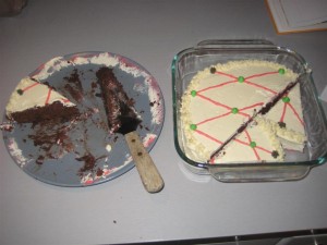