Summary sheet of ways to map statistical uncertainty

A few years ago, a team at the Cornell Program on Applied Demographics (PAD) created a really nice demo of several ways to show statistical uncertainty on thematic maps / choropleths. They have kindly allowed me to host their large file here: PAD_MappingExample.pdf (63 MB)

Screenshot of index page from PAD mapping examples

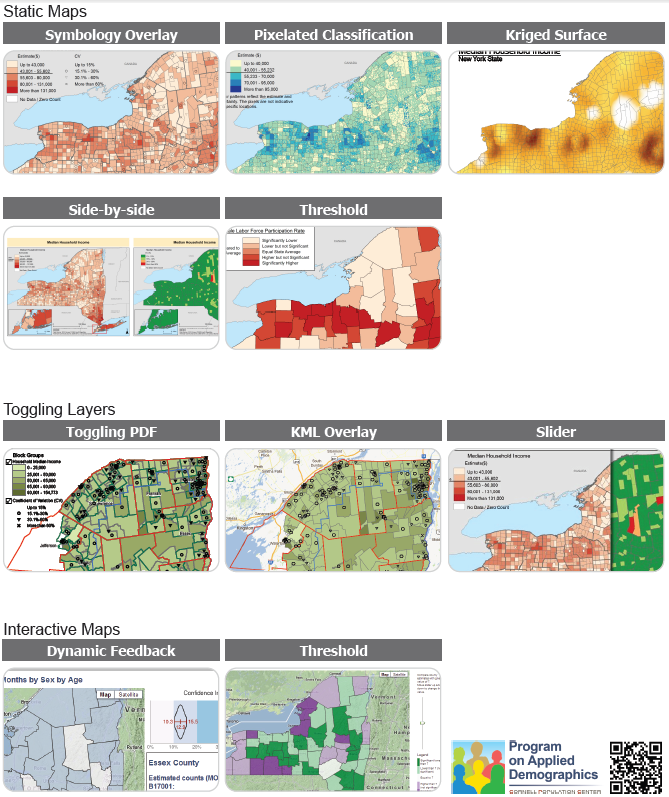
Each of these maps shows a dataset with statistical estimates and their precision/uncertainty for various areas in New York state. If we use color or shading to show the estimates, like in a traditional choropleth map, how can we also show the uncertainty at the same time? The PAD examples include several variations of static maps, interaction by toggling overlays, and interaction with mouseover and sliders. Interactive map screenshots are linked to live demos on the PAD website.

I’m still fascinated by this problem. Each of these approaches has its strengths and weaknesses: Symbology Overlay uses separable dimensions, but there’s no natural order to the symbols. Pixelated Classification seems intuitively clear, but may be misleading if people (incorrectly) try to find meaning in the locations of pixels within an area. Side-by-side maps are each clear on their own, but it’s hard to see both variables at once. Dynamic Feedback gives detailed info about precision, but only for one area at a time, not all at once. And so forth. It’s an interesting challenge, and I find it really helpful to see so many potential solutions collected in one document.

The creators include Nij Tontisirin and Sutee Anantsuksomsri (both since moved on from Cornell), and Jan Vink and Joe Francis (both still there). The pixellated classification map is based on work by Nicholas Nagle.

For more about mapping uncertainty, see their paper:

Francis, J., Tontisirin, N., Anantsuksomsri, S., Vink, J., & Zhong, V. (2015). Alternative strategies for mapping ACS estimates and error of estimation. In Hoque, N. and Potter, L. B. (Eds.), Emerging Techniques in Applied Demography (pp. 247–273). Dordrecht: Springer Netherlands, DOI: 10.1007/978-94-017-8990-5_16 [preprint]

and my related posts:

Localized Comparisons: my own attempts at showing uncertainty in an interactive map and in a cartogram, plus links to work by Gabriel Florit, David Sparks, Nicholas Nagle, and Nancy Torrieri & David Wong
Nice example of a map with uncertainty: a map by Michael Wininger

See also Visualizing Attribute Uncertainty in the ACS: An Empirical Study of Decision-Making with Urban Planners. This talk by Amy Griffin is about studying how urban planners actually use statistical uncertainty on maps in their work.

About to teach Statistical Graphics and Visualization course at CMU

I’m pretty excited for tomorrow: I’ll begin teaching the Fall 2015 offering of 36-721, Statistical Graphics and Visualization. This is a half-semester course designed primarily for students in our MSP program (Masters in Statistical Practice).

A large part of the focus will be on useful principles and frameworks: human visual perception, the Grammar of Graphics, graphic design and interaction design, and more current dataviz research. As for tools, besides base R and ggplot2, I’ll introduce a bit of Tableau, D3.js, and Inkscape/Illustrator. For assessments, I’m trying a variant of “specs grading”, with a heavy use of rubrics, hoping to make my expectations clear and my TA’s grading easier.

Di Cook, LDA and CART classification boundaries on Flea Beetles dataset — Classifier diagnostics from Cook & Swayne’s book

My initial course materials are up on my department webpage.
Here are the

syllabus (pdf),
first lecture (pdf created with Rmd), and
first homework (pdf) with dataset (csv).

(I’ll probably just use Blackboard during the semester, but I may post the final materials here again.)

It’s been a pleasant challenge to plan a course that can satisfy statisticians (slice and dice data quickly to support detailed analyses! examine residuals and other model diagnostics! work with data formats from rectangular CSVs through shapefiles to social networks!) … while also passing on lessons from the data journalism and design communities (take design and the user experience seriously! use layout, typography, and interaction sensibly!). I’m also trying to put into practice all the advice from teaching seminars I’ve taken at CMU’s Eberly Center.

Also, in preparation, this summer I finally enjoyed reading more of the classic visualization books on my list.

Cleveland’s The Elements of Graphing Data and Robbins’ Creating More Effective Graphs are chock full of advice on making clear graphics that harness human visual perception correctly.
Ware’s Information Visualization adds to this the latest research findings and a ton of useful detail.
Cleveland’s Visualizing Data and Cook & Swayne’s Interactive and Dynamic Graphics for Data Analysis are a treasure trove of practical data analysis advice. Cleveland’s many case studies show how graphics are a critical part of exploratory data analysis (EDA) and model-checking. In several cases, his analysis demonstrates that previously-published findings used an inappropriate model and reached poor conclusions due to what he calls rote data analysis (RDA). Cook & Swayne do similar work with more modern statistical methods, including the first time I’ve seen graphical diagnostics for many machine learning tools. There’s also a great section on visualizing missing data. The title is misleading: you don’t need R and GGobi to learn a lot from their book.
Monmonier’s How to Lie with Maps refers to dated technology, but the concepts are great. It’s still useful to know just how maps are made, and how different projections work and why it matters. Much of cartographic work sounds analogous to statistical work: making simplifications in order to convey a point more clearly, worrying about data quality and provenance (different areas on the map might have been updated by different folks at different times), setting national standards that are imperfect but necessary… The section on “data maps” is critical for any statistician working with spatial data, and the chapter on bureaucratic mapping agencies will sound familiar to my Census Bureau colleagues.

I hope to post longer notes on each book sometime later.

One more difference between statistics and [machine learning, data science, etc.]

Statisticians have always done a myriad of different things related to data collection and analysis. Many of us are surprised (even frustrated) that Data Science is even a thing. “That’s just statistics under a new name!” we cry. Others are trying to bring Data Science, Machine Learning, Data Mining, etc. into our fold, hoping that Statistics will be the “big tent” for everyone learning from data.

But I do think there is one core thing that differentiates Statisticians from these others. Having an interest in this is why you might choose to major in statistics rather than applied math, machine learning, etc. And it’s the reason you might hire a trained statistician rather than someone else fluent with data:

Statisticians use the idea of variability due to sampling to design good data collection processes, to quantify uncertainty, and to understand the statistical properties of our methods.

When applied statisticians design an experiment or a survey, they account for the inherent randomness and try to control it. They plan your study in such a way that’ll make your estimates/predictions as accurate as possible for the sample size you can afford. And when they analyze the data, alongside each estimate they report its precision, so you can decide whether you have enough evidence or whether you still need further study. For more complex models, they also worry about overfitting: can this model generalize well to the population, or is too complicated to estimate with this sample and hence is it just fitting noise?

When theoretical statisticians invent a new estimator, they study how well it’ll perform over repeated sampling, under various assumptions. They study its statistical properties first and foremost. Loosely speaking: How variable will the estimates tend to be? Will they be biased (i.e. tend to always overestimate or always underestimate)? How robust will they be to outliers? Is the estimator consistent (as the sample size grows, does the estimate tend to approach the true value)?

These are not the only important things in working with data, and they’re not the only things statisticians are trained to do. But (as far as I can tell) they are a much deeper part of the curriculum in statistics training than in any other field. Statistics is their home. Without them, you can often still be a good data analyst but a poor statistician.

Continue reading “One more difference between statistics and [machine learning, data science, etc.]” →

Dataviz contest on “Visualizing Well-Being”

Someone from OECD emailed me about a data visualization contest for the Wikiprogress website (the deadline is August 24th):

I am contacting you on behalf of the website Wikiprogress, which is currently running a Data Visualization Contest, with the prize of a paid trip to Mexico to attend the 5th OECD World Forum in Guadalajara in October this year. Wikiprogress is an open-source website, hosted by the OECD, to facilitate the exchange of information on well-being and sustainability, and the aim of the competition is to encourage participants to use well-being measurement in innovative ways to a) show how data on well-being give a more meaningful picture of the progress of societies than more traditional growth-oriented approaches, and b) to use their creativity to communicate key ideas about well-being to a broad audience.

After reading your blog, I think that you and your readers might be interested in this challenge. The OECD World Forums bring together hundreds of change-makers from around the world, from world leaders to small, grassroots projects, and the winners will have their work displayed and will be presented with a certificate of recognition during the event.

You can also visit the competition website here: http://bit.ly/1Gsso2y

It does sound like a challenge that might intrigue this blog’s readers:

think about how to report human well-being, beyond traditional measures like GDP;
find relevant good datasets (“official statistics” or otherwise);
visualize these measures’ importance or insightful trends in the data; and
possibly win a prize trip to the next OECD forum in Guadalajara, Mexico to network with others who are interested in putting data, statistics, and visualization to good use.

“Don’t invert that matrix” – why and how

The first time I read John Cook’s advice “Don’t invert that matrix,” I wasn’t sure how to follow it. I was familiar with manipulating matrices analytically (with pencil and paper) for statistical derivations, but not with implementation details in software. For reference, here are some simple examples in MATLAB and R, showing what to avoid and what to do instead.

[Edit: R code examples and results have been revised based on Nicholas Nagle’s comment below and advice from Ryan Tibshirani. See also a related post by Gregory Gundersen.]

If possible, John says, you should just ask your scientific computing software to directly solve the linear system $Ax = b$ . This is often faster and more numerically accurate than computing the matrix inverse of A and then computing $x = A^{-1}b$ .

We’ll chug through a computation example below, to illustrate the difference between these two methods. But first, let’s start with some context: a common statistical situation where you may think you need matrix inversion, even though you really don’t.

[One more edit: I’ve been guilty of inverting matrices directly, and it’s never caused a problem in my one-off data analyses. As Ben Klemens comments below, this may be overkill for most statisticians. But if you’re writing a package, which many people will use on datasets of varying sizes and structures, it may well be worth the extra effort to use solve or QR instead of inverting a matrix if you can help it.]

Continue reading ““Don’t invert that matrix” – why and how” →

Two principled approaches to data visualization

Yesterday I spoke at Stat Bytes, our student-run statistical computing seminar.

My goal was to introduce two principled frameworks for thinking about data visualization: human visual perception and the Grammar of Graphics.
(We also covered some relevant R packages: RColorBrewer, directlabels, and a gentle intro to ggplot2.)

These are not the only “right” approaches, nor do they guarantee your graphics will be good. They are just useful tools to have in your arsenal.

Example plot with direct labels and ColorBrewer colors, made in ggplot2.

The talk was also a teaser for my upcoming fall course, 36-721: Statistical Graphics and Visualization [draft syllabus pdf].

Here are my

The talk was quite interactive, so the slides aren’t designed to stand alone. Open the slides and follow along using my notes below.
(Answers are intentionally in white text, so you have a chance to think for yourself before you highlight the text to read them.)

If you want a deeper introduction to dataviz, including human visual perception, Alberto Cairo’s The Functional Art [website, amazon] is a great place to start.
For a more thorough intro to ggplot2, see creator Hadley Wickham’s own presentations at the bottom of this page.

Continue reading “Two principled approaches to data visualization” →

Simplistic thinking in statistical inference

My friend Brian Segal, at the University of Michigan, writes in response to the journal that banned statistical inference:

If nothing else, I think BASP did a great job of starting a discussion on p-values, and more generally, the role of statistical inference in certain types of research. Stepping back a bit, I think the discussion fits into a broader question of how we deal with answers that are inherently grey, as opposed to clear cut. Hypothesis testing, combined with traditional cutoff values, is a neat way to get a yes/no answer, but many reviewers want a yes/no answer, even in the absence of hypothesis tests.

As one example, I recently helped a friend in psychology to validate concepts measured by a survey. In case you haven’t done this before, here’s a quick (and incomplete) summary of construct validation: based on substantive knowledge, group the questions in the survey into groups, each of which measures a different underlying concept, like positive attitude, or negativity. The construct validation question is then, “Do these groups of questions actually measure the concepts I believe they measure?”

In addition to making sure the groups are defensible based on their interpretation, you usually have to do a quantitative analysis to get published The standard approach is to model the data with a structural equation model (as a side note, this includes confirmatory factor analysis, which is not factor analysis!). The goodness of fit statistic is useless in this context, because the null hypothesis is not aligned with the scientific question, so people use a variety of heuristics, or fit indices, to decide if the model fits. The model is declared to either fit or not fit (and consequently the construct is either valid or not valid) depending on whether the fit index is larger or smaller than a rule-of-thumb value. This is the same mentality as hypothesis testing.

Setting aside the question of whether it makes sense to use structural equation models to validate constructs, the point I’m trying to make is that the p-value mentality is not restricted to statistical inference. Like any unsupervised learning situation, it’s very difficult to say how well the hypothesized groups measure the underlying constructs (or if they even exist). Any answer is inherently grey, and yet many researchers want a yes/no answer. In these types of cases, I think it would be great if statisticians could help other researchers come to terms not just with the limits of the statistical tools, but with the inquiry itself.

I agree with Brian that we can all do a better job of helping our collaborators to think statistically. Statistics is not just a set of arbitrary yes/no hoops to jump through in the process of publishing a paper; it’s a kind of applied epistemology. As tempting as it might be to just ban all conclusions entirely, we statisticians are well-trained in probing what can be known and how that knowledge can be justified. Give us the chance, and we’d would love to help you navigate the subtleties, limits, and grey areas in your research!

DotCity: a game written in R? and other statistical computer games?

A while back I recommended Nathan Uyttendaele’s beginner’s guide to speeding up R code.

I’ve just heard about Nathan’s computer game project, DotCity. It sounds like a statistician’s minimalist take on SimCity, with a special focus on demographic shifts in your population of dots (baby booms, aging, etc.). Furthermore, he’s planning to program the internals using R.

This is where scatterplot points go to live and play when they're not on duty. — This is where scatterplot points go to live and play when they’re not on duty.

Consider backing the game on Kickstarter (through July 8th). I’m supporting it not just to play the game itself, but to see what Nathan learns from the development process. How do you even begin to write a game in R? Will gamers need to have R installed locally to play it, or will it be running online on something like an RStudio server?

Meanwhile, do you know of any other statistics-themed computer games?

I missed the boat on backing Timmy’s Journey, but happily it seems that development is going ahead.
SpaceChem is a puzzle game about factory line optimization (and not, actually, about chemistry). Perhaps someone can imagine how to take it a step further and gamify statistical process control à la Shewhart and Deming.
It’s not exactly stats, but working with data in textfiles is an important related skill. The Command Line Murders is a detective noir game for teaching this skill to journalists.
The command line approach reminds me of Zork and other old text adventure / interactive fiction games. Perhaps, using a similar approach to the step-by-step interaction of swirl (“Learn R, in R”), someone could make an I.F. game about data analysis. Instead of OPEN DOOR, ASK TROLL ABOUT SWORD, TAKE AMULET, you would type commands like READ TABLE, ASK SCIENTIST ABOUT DATA DICTIONARY, PLOT RESIDUALS… all in the service of some broader story/puzzle context, not just an analysis by itself.
Kim Asendorf wrote a fictional “short story” told through a series of data visualizations. (See also FlowingData’s overview.) The same medium could be used for a puzzle/mystery/adventure game.

After 4th semester of statistics PhD program

This was my first PhD semester without any required courses (more or less). That means I had time to focus on research, right?

It was also my first semester as a dad. Exhilarating, joyful, and exhausting 🙂 So, time was freed up by having less coursework, but it was reallocated largely towards diapering and sleep. Still, I did start on a new research project, about which I’m pretty excited.

Our department was also recognized as one of the nation’s fastest-growing statistics departments. I got to see some of the challenges with this first-hand as a TA for a huge 200-student class.

See also my previous posts on the 1st, the 2nd, and the 3rd semesters of my Statistics PhD program.

Classes:

Statistical Computing:
This was a revamped, semi-required, half-semester course, and we were the guinea pigs. I found it quite useful. The revamp was spearheaded by our department chair Chris Genovese, who wanted to pass on his software engineering knowledge/mindset to the rest of us statisticians. This course was not just “how to use R” (though we did cover some advanced topics from Hadley Wickham’s new books Advanced R and R Packages; and it got me to try writing homework assignment analyses as R package vignettes).
Rather, it was a mix of pragmatic coding practices (using version control such as Git; writing and running unit tests; etc.) and good-to-know algorithms (hashing; sorting and searching; dynamic programming; etc.). It’s the kind of stuff you’d pick up on the job as a programmer, or in class as a CS student, but not necessarily as a statistician even if you write code often.
The homework scheme was nice in that we could choose from a large set of assignments. We had to do two per week, but could do them in any order—so you could do several on a hard topic you really wanted to learn, or pick an easy one if you were having a rough week. The only problem is that I never had to practice certain topics if I wanted to avoid them. I’d like to try doing this as an instructor sometime, but I’d want to control my students’ coverage a bit more tightly.
This fall, Stat Computing becomes an actually-required, full-semester course and will be cotaught by my classmate Alex Reinhart.
Convex Optimization:
Another great course with Ryan Tibshirani. Tons of work, with fairly long homeworks, but I also learned a huge amount of very practical stuff, both theory (how to prove a certain problem is convex? how to prove a certain optimization method works well?) and practice (which methods are likely to work on which problems?).
My favorite assignments were the ones in which we replicated analyses from recent papers. A great way to practice your coding, improve your optimization, and catch up with the literature all at once. One of these homeworks actually inspired in me a new methodological idea, which I’ve pursued as a research project.
Ryan’s teaching was great as usual. He’d start each class with a review from last time and how it connects to today. There were also daily online quizzes, posted after class and due at midnight, that asked simple comprehension questions—not difficult and not a huge chunk of your grade, but enough to encourage you to keep up with the class regularly instead of leaving your studying to the last minute.
TAing for Intro to Stat Inference:
This was the 200-student class. I’m really glad statistics is popular enough to draw such crowds, but it’s the first time the department has had so many folks in the course, and we are still working out how to manage it. We had an army of undergrad- and Masters-level graders for the weekly homeworks, but just three of us PhD-level TAs to grade midterms and exams, which made for several loooong weekends.
I also regret that I often wasn’t at my best during my office hours this semester. I’ll blame it largely on baby-induced sleep deprivation, but I could have spent more time preparing too. I hope the students who came to my sessions still found them helpful.
Next semester, I’ll be teaching the grad-level data visualization course! It will be heavily inspired by Alberto Cairo’s book and his MOOC. I’m still trying to find the right balance between the theory I think is important (how does the Grammar of Graphics work, and why does it underpin ggplot2, Tableau, D3, etc.? how does human visual perception work? what makes for a well-designed graphic?) vs. the tool-using practice that would certainly help many students too (teach me D3 and Shiny so I can make something impressive for portfolios and job interviews!)
I was glad to hear Scott Murray’s reflections on his recent online dataviz course co-taught with Alberto.

Research:

Sparse PCA: I’ve been working with Jing Lei on several aspects of sparse PCA, extending some methodology that he’s developed with collaborators including his wife Kehui Chen (also a statistics professor, just down the street at UPitt). It’s a great opportunity to practice what I’ve learned in Convex Optimization and earlier courses. I admired Jing’s teaching when I took his courses last year, and I’m enjoying research work with him: I have plenty of independence, but he is also happy to provide direction and advice when needed.
We have some nice simulation results illustrating that our method can work in an ideal setting, so now it’s time to start looking at proofs of why it should work 🙂 as well as a real dataset to showcase its use. More on this soon, I hope.
Unfortunately, one research direction that I thought could become a thesis topic turned out to be a dead end as soon as we formulated the problem more precisely. Too bad, though at least it’s better to find out now than after spending months on it.
I still need to finish writing up a few projects from last fall: my ADA report and a Small Area Estimation paper with Rebecca Steorts (now moving from CMU to Duke). I really wish I had pushed myself to finish them before the baby came—now they’ve been on the backburner for months. I hope to wrap them up this summer. Apologies to my collaborators!

Life:

Being a sDADistician: Finally, my penchant for terrible puns becomes socially acceptable, maybe even expected—they’re “dad jokes,” after all.
Grad school seems to be a good time to start a family. (If you don’t believe me, I heard it as well from Rob Tibshirani last semester.) I have a pretty flexible schedule, so I can easily make time to see the baby and help out, working from home or going back and forth, instead of staying all day on campus or at the office until late o’clock after he’s gone to bed. Still, it helps to make a concrete schedule with my wife, about who’s watching the baby when. Before he arrived, I had imagined we could just pop him in the crib to sleep or entertain himself when we needed to work—ah, foolish optimism…
It certainly doesn’t work for us both to work from home and be half-working, half-watching him. Neither the work nor the child care is particularly good that way. But when we set a schedule, it’s great for organization & motivation—I only have a chunk of X hours now, so let me get this task DONE, not fritter the day away.
I’ve spent less time this semester attending talks and department events (special apologies to all the students whose defenses I missed!), but I’ve also forced myself to get much better about ignoring distractions like computer games and Facebook, and I spend more of my free time on things that really do make me feel better such as exercise and reading.
Stoicism: This semester I decided to really finish the Seneca book I’d started years ago. It is part of a set of philosophy books I received as a gift from my grandparents. Long story short, once I got in the zone I was hooked, and I’ve really enjoyed Seneca’s Letters to Lucilius as well as Practical Philosophy, a Great Courses lecture series on his contemporaries.
It turns out several of my fellow students (including Lee Richardson) have been reading the Stoics lately too. The name “Stoic” comes from “Stoa,” i.e. porch, after the place where they used to gather… so clearly we need to meet for beers at The Porch by campus to discuss this stuff.
Podcasts: This semester I also discovered the joy of listening to good podcasts.
(1) Planet Money is the perfect length for my walk to/from campus, covers quirky stories loosely related to economics and finance, and includes a great episode with a shoutout to CMU’s Computer Science school.
(2) Talking Machines is a more academic podcast about Machine Learning. The hosts cover interesting recent ideas and hit a good balance—the material is presented deeply enough to interest me, but not so deeply I can’t follow it while out on a walk. The episodes usually explain a novel paper and link to it online, then answer a listener question, and end with an interview with a ML researcher or practitioner. They cover not only technical details, but other important perspectives as well: how do you write a ML textbook and get it published? how do you organize a conference to encourage women in ML? how do you run a successful research lab? Most of all, I love that they respect statisticians too 🙂 and in fact, when they interview the creator of The Automatic Statistician, they probe him on whether this isn’t just going to make the data-fishing problem worse.
(3) PolicyViz is a new podcast on data visualization, with somewhat of a focus on data and analyses for the public: government statistics, data journalism, etc. It’s run by Jon Schwabish, whom I (think I) got to meet when I still worked in DC, and whose visualization workshop materials are a great resource.
It’s a chore to update R with all the zillion packages I have installed. I found that Tal Galili’s installr manages updates cleanly and helpfully.
Next time I bake brownies, I’ll add some spices and call them “Chai squares.” But we must ask, of course: what size to cut them for optimal goodness of fit in the mouth?

Next up: the 5th, 6th, 7th, 8th, 9th, and 10th semesters of my Statistics PhD program.

Nice example of a map with uncertainty

OK, back to statistics and datavis.

As I’ve said before, I’m curious about finding better ways to draw maps which simultaneously show numerical estimates and their precision or uncertainty.

The April 2015 issue of Significance magazine includes a nice example of this [subscription link; PDF], thanks to Michael Wininger. Here is his Figure 2a (I think the labels for the red and blue areas are mistakenly swapped, but you get the idea):

Basically, Wininger is mapping the weather continuously over space, and he overlays two contours: one for where the predicted snowfall amount is highest, and another for where the probability of snowfall is highest.

I can imagine people would also enjoy an interactive version of this map, where you have sliders for the two cutoffs (how many inches of snow? what level of certainty?). You could also just show more levels of the contours on one static map, by adding extra lines, though that would get messy fast.

I think Wininger’s approach looks great and is easy to read, but it works largely because he’s mapping spatially-continuous data. The snowfall levels and their certainties are estimated at a very fine spatial resolution, unlike say a choropleth map of the average snowfall by county or by state. The other thing that helps here is that certainty is expressed as a probability (which most people can interpret)… not as a measure of spread or precision (standard deviation, margin of error, coefficient of variation, or what have you).

Could this also work on a choropleth map? If you only have data at the level of discrete areas, such as counties… Well, this is not a problem with weather data, but it does come up with administrative or survey data. Say you have survey estimates for the poverty rate in each county (along with MOEs or some other measure of precision). You could still use one color to fill all the counties with high estimated poverty rates. Then use another color to fill all the counties with highly precise estimates. Their overlap would show the areas where poverty is estimated to be high and that estimate is very precise. Sliders would let the readers set their own definition of “high poverty” and “highly precise.”

I might be wrong, but I don’t think I’ve seen this approach before. Could be worth a try.