Stefan Wager on the statistics of random forests

Yesterday’s CMU stats department seminar was given by Stefan Wager, who spoke on statistical estimation with random forests (RFs).

Random forests are very popular models in machine learning and data science for prediction tasks. They often have great empirical performance when all you need is a black-box algorithm, as in many Kaggle competitions. On the other hand, RFs are less commonly used for estimation tasks, because historically we could not do well at computing confidence intervals or hypothesis tests: there was no good understanding of RFs’ statistical properties, nor good estimators of variance (needed for confidence intervals). Until now.

Wager has written several papers on the statistical properties of random forests. He also has made code available for computing pointwise confidence intervals. (Confidence bands, for the whole RF-estimated regression function at once, have not been developed yet.)

Wager gave concrete examples of when this can be useful, for instance in personalized medicine. You don’t always want just point-estimate predictions for how a patient will respond to a certain treatment. Often you want some margin of error too, so you can decide on the treatment that’s most likely to help. That is, you’d like to avoid a treatment with a positive estimate but a margin of error so big that we’re not sure it helps (it might actually be harmful).

It’s great to see such work on statistical properties of (traditionally) black-box models. In general, it’s an exciting (if challenging) problem to figure out properties and estimate MOEs for such ML-flavored algorithms. Some data science or applied ML folks like to deride high-falutin’ theoretical statisticians, as did Breiman himself (the originator of random forests)… But work like Wager’s is very practical, not merely theoretically interesting. We need more of this, not less.

PS—One other nifty idea from his talk, something I hadn’t seen before: In the usual k-nearest-neighbor algorithm, you pick a target point where you want to make a prediction, then use Euclidean distance to find the k closest neighbors in the training data. Wager showed examples where it works better to train a random forest first, then use “number of trees where this data point is in the same leaf as the target point” as your distance. That is, choose as “neighbors” any points that tend to land in the same leaf as your target, regardless of their Euclidean distance. The results seem more stable than usual kNN. New predictions may be faster to compute too.

Followup for myself:

  • Ryan Tibshirani asked about using shrinkage together with random forests. I can imagine small area estimators that shrink towards a CART or random forest prediction instead of a usual regression, but Ryan sounded more like he had lasso or ridge penalties in mind. Does anyone do either of these?
  • Trees and forests can only split perpendicular to the variables, but sometimes you might have “rotated” structure (i.e. interesting clustering splits are diagonal in the predictor space). So, do people ever find it useful to do PCA first, and *then* CART or RFs? Maybe even using all the PCs, so that you’re not doing it for dimension reduction, just for the sake of rotation? Or maybe some kind of sparse PCA variant where you only rotate certain variables that need it, but leave the others alone (unrotated) when you run CART or RFs?
  • The “infinitesimal jackknife” sounded like a nifty proof technique, but I didn’t catch all the details. Read up more on this.

Participant observation in statistics classes (Steve Fienberg interview)

CMU professor Steve Fienberg has a nice recent interview at Statistics Views.

He brings up great nuggets of stats history, including insights into the history and challenges of Big Data. I also want to read his recommended books, especially Fisher’s Design of Experiments and Raiffa & Schlaifer’sApplied Statistical Decision Theory. But my favorite part was about involving intro stats students in data collection:

One of the things I’ve been able to do is teach a freshman seminar every once in a while. In 1990, I did it as a class in a very ad hoc way and then again in 2000, and again in 2010, I taught small freshman seminars on the census. Those were the census years, so I would bring real data into the classroom which we would discuss. One of the nice things about working on those seminars is that, because I personally knew many of the Census Directors, I was able to bring many of them to class as my guests. It was great fun and it really changes how students think about what they do. In 1990, we signed all students up as census enumerators and they did a shelter and homeless night and had to come back and describe their experiences and share them. That doesn’t sound like it should belong in a stat class but I can take you around here at JSM and introduce you to people who were in those classes and they’ve become statisticians!

What a great teaching idea 🙂 It reminds me of discussions in an anthropology class I took, where we learned about participant observation and communities of practice. Instead of just standing in a lecture hall talking about statistics, we’d do well to expose students to real-life statistical work “in the field”—not just analysis, but data collection too. I still feel strongly that data collection/generation is the heart of statistics (while data analysis is just icing on the cake), and Steve’s seminar is a great way to hammer that home.

Victoria Stodden on Reproducible Research

Yesterday’s department seminar was by Victoria Stodden [see slides from Nov 9, 2015]. With some great Q&A during the talk, we only made it through about half the slides.

Dr Stodden spoke about several kinds of reproducibility important to science, and their links to different “flavors” of science. As I understood it, there are

  • empirical reproducibility: are the methods (lab-bench protocol, psych-test questionnaire, etc.) available, so that we could repeat the experiment or data-collection?
  • computational reproducibility: are the code and data available, so that we could repeat the processing and calculations?
  • statistical reproducibility: was the sample large enough that we can expect to get comparable results, if we do repeat the experiment and calculations?

Her focus is on the computational piece. As more and more research involves methodological contributions primarily in the software itself (and not explained in complete detail in the paper), it’s critical for that code to be open and reproducible.

Continue reading “Victoria Stodden on Reproducible Research”

Teaching data visualization: approaches and syllabi

While I’m still working on my reflection of the dataviz course I just taught, there were some useful dataviz-teaching talks at the recent IEEE VIS conference.

Jen Christiansen and Robert Kosara have great summaries of the panel on “Vis, The Next Generation: Teaching Across the Researcher-Practitioner Gap.”

Even better, slides are available for some of the talks: Marti Hearst, Tamara Munzner, and Eytan Adar. Lots of inspiration for the next time I teach.

Hearst_ClassDiscussions

Finally, here are links to the syllabi or websites of various past dataviz courses. Browsing these helps me think about what to cover and how to teach it.

Update: More syllabi shared through the Isostat mailing list:

Not quite data visualization, but related:

Comment below or tweet @civilstat with any others I’ve missed, and I’ll add them to the list.
(Update: Thanks to John Stasko for links to many I missed, including his own excellent course site & resource page.)

Why bother with magrittr

I’ve seen R users swooning over the magrittr package for a while now, but I couldn’t make heads or tails of all these scary %>% symbols. Finally I had time for a closer look, and it seems potentially handy indeed. Here’s the idea and a simple toy example.

So, it can be confusing and messy to write (and read) functions from the inside out. This is especially true when functions take multiple arguments. Instead, magrittr lets you write (and read) functions from left to right.

Say you need to compute the LogSumExp function \log\left(\sum_{i=1}^n\exp(x_i)\right)
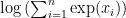
, and you’d like your code to specify the logarithm base explicitly.

In base R, you might write
log(sum(exp(MyData)), exp(1))
But this is a bit of a mess to read. It takes a lot of parentheses-matching to see that the exp(1) is an argument to log and not to one of the other functions.

Instead, with magrittr, you program from left to right:
MyData %>% exp %>% sum %>% log(exp(1))
The pipe operator %>% takes output from the left and uses it as the first argument of input on the right. Now it’s very clear that the exp(1) is an argument to log.

There’s a lot more you can do with magrittr, but code with fewer nested parentheses is already a good selling point for me.

Apart from cleaning up your nested functions, this approach to programming might be helpful if you write a lot of JavaScript code, for example if you make D3.js visualizations. R’s magrittr pipe is similar in spirit to JavaScript’s method chaining, so it might make context-switching a little easier.

Statistical Graphics and Visualization course materials

I’ve just finished teaching the Fall 2015 session of 36-721, Statistical Graphics and Visualization. Again, it is a half-semester course designed primarily for students in the MSP program (Masters of Statistical Practice) in the CMU statistics department. I’m pleased that we also had a large number of students from other departments taking this as an elective.

For software we used mostly R (base graphics, ggplot2, and Shiny). But we also spent some time on Tableau, Inkscape, D3, and GGobi.

We covered a LOT of ground. At each point I tried to hammer home the importance of legible, comprehensible graphics that respect human visual perception.

Pie chart with remake
Remaking pie charts is a rite of passage for statistical graphics students

My course materials are below. Not all the slides are designed to stand alone, but I have no time to remake them right now. I’ll post some reflections separately.

Download all materials as a ZIP file (38 MB), or browse individual files:
Continue reading “Statistical Graphics and Visualization course materials”

Chai Squares

I saw this typo for Chi Square a while back and thought it’d make a great recipe idea. Turns out I was right: these bars won a prize at my department’s World Statistics Day bake-off.

ChaiSquares

Start with Mark Bittman’s blondie recipe (copied/adapted from here), and add some of the spices that go into chai tea.

  • 8 tablespoons (1 stick, 4 ounces or 113 grams) butter, melted
  • 1 cup (218 grams or 7 3/4 ounces for light; 238 grams or 8 3/8 ounces for dark) brown sugar
  • 1 large egg
  • 1 teaspoon vanilla
  • Pinch salt
  • 1 cup (4 3/8 ounces or 125 grams) all-purpose flour
  • 1/2 teaspoon cardamom
  • 1/2 teaspoon cinnamon
  • 1/2 teaspoon ground ginger
  • 1/2 teaspoon ground cloves
  • scant 1/2 teaspoon fresh ground black pepper
  1. Preheat oven to 350°F. Butter an 8×8 pan, or line the pan with aluminum foil and grease the foil.
  2. Mix melted butter with brown sugar. Beat until smooth. Beat in egg and vanilla.
  3. Combine salt, flour, and spices. Gently stir flour mixture into butter mixture.
  4. Pour into prepared pan. Bake 20-25 minutes, or until barely set in the middle. Cool on rack before cutting them.

Enjoy!

Summary sheet of ways to map statistical uncertainty

A few years ago, a team at the Cornell Program on Applied Demographics (PAD) created a really nice demo of several ways to show statistical uncertainty on thematic maps / choropleths. They have kindly allowed me to host their large file here: PAD_MappingExample.pdf (63 MB)

Screenshot of index page from PAD mapping examples

Each of these maps shows a dataset with statistical estimates and their precision/uncertainty for various areas in New York state. If we use color or shading to show the estimates, like in a traditional choropleth map, how can we also show the uncertainty at the same time? The PAD examples include several variations of static maps, interaction by toggling overlays, and interaction with mouseover and sliders. Interactive map screenshots are linked to live demos on the PAD website.

I’m still fascinated by this problem. Each of these approaches has its strengths and weaknesses: Symbology Overlay uses separable dimensions, but there’s no natural order to the symbols. Pixelated Classification seems intuitively clear, but may be misleading if people (incorrectly) try to find meaning in the locations of pixels within an area. Side-by-side maps are each clear on their own, but it’s hard to see both variables at once. Dynamic Feedback gives detailed info about precision, but only for one area at a time, not all at once. And so forth. It’s an interesting challenge, and I find it really helpful to see so many potential solutions collected in one document.

The creators include Nij Tontisirin and Sutee Anantsuksomsri (both since moved on from Cornell), and Jan Vink and Joe Francis (both still there). The pixellated classification map is based on work by Nicholas Nagle.

For more about mapping uncertainty, see their paper:

Francis, J., Tontisirin, N., Anantsuksomsri, S., Vink, J., & Zhong, V. (2015). Alternative strategies for mapping ACS estimates and error of estimation. In Hoque, N. and Potter, L. B. (Eds.), Emerging Techniques in Applied Demography (pp. 247–273). Dordrecht: Springer Netherlands, DOI: 10.1007/978-94-017-8990-5_16 [preprint]

and my related posts:

See also Visualizing Attribute Uncertainty in the ACS: An Empirical Study of Decision-Making with Urban Planners. This talk by Amy Griffin is about studying how urban planners actually use statistical uncertainty on maps in their work.

About to teach Statistical Graphics and Visualization course at CMU

I’m pretty excited for tomorrow: I’ll begin teaching the Fall 2015 offering of 36-721, Statistical Graphics and Visualization. This is a half-semester course designed primarily for students in our MSP program (Masters in Statistical Practice).

A large part of the focus will be on useful principles and frameworks: human visual perception, the Grammar of Graphics, graphic design and interaction design, and more current dataviz research. As for tools, besides base R and ggplot2, I’ll introduce a bit of Tableau, D3.js, and Inkscape/Illustrator. For assessments, I’m trying a variant of “specs grading”, with a heavy use of rubrics, hoping to make my expectations clear and my TA’s grading easier.

Di Cook, LDA and CART classification boundaries on Flea Beetles dataset
Classifier diagnostics from Cook & Swayne’s book

My initial course materials are up on my department webpage.
Here are the

  • syllabus (pdf),
  • first lecture (pdf created with Rmd), and
  • first homework (pdf) with dataset (csv).

(I’ll probably just use Blackboard during the semester, but I may post the final materials here again.)

It’s been a pleasant challenge to plan a course that can satisfy statisticians (slice and dice data quickly to support detailed analyses! examine residuals and other model diagnostics! work with data formats from rectangular CSVs through shapefiles to social networks!) … while also passing on lessons from the data journalism and design communities (take design and the user experience seriously! use layout, typography, and interaction sensibly!). I’m also trying to put into practice all the advice from teaching seminars I’ve taken at CMU’s Eberly Center.

Also, in preparation, this summer I finally enjoyed reading more of the classic visualization books on my list.

  • Cleveland’s The Elements of Graphing Data and Robbins’ Creating More Effective Graphs are chock full of advice on making clear graphics that harness human visual perception correctly.
  • Ware’s Information Visualization adds to this the latest research findings and a ton of useful detail.
  • Cleveland’s Visualizing Data and Cook & Swayne’s Interactive and Dynamic Graphics for Data Analysis are a treasure trove of practical data analysis advice. Cleveland’s many case studies show how graphics are a critical part of exploratory data analysis (EDA) and model-checking. In several cases, his analysis demonstrates that previously-published findings used an inappropriate model and reached poor conclusions due to what he calls rote data analysis (RDA). Cook & Swayne do similar work with more modern statistical methods, including the first time I’ve seen graphical diagnostics for many machine learning tools. There’s also a great section on visualizing missing data. The title is misleading: you don’t need R and GGobi to learn a lot from their book.
  • Monmonier’s How to Lie with Maps refers to dated technology, but the concepts are great. It’s still useful to know just how maps are made, and how different projections work and why it matters. Much of cartographic work sounds analogous to statistical work: making simplifications in order to convey a point more clearly, worrying about data quality and provenance (different areas on the map might have been updated by different folks at different times), setting national standards that are imperfect but necessary… The section on “data maps” is critical for any statistician working with spatial data, and the chapter on bureaucratic mapping agencies will sound familiar to my Census Bureau colleagues.

I hope to post longer notes on each book sometime later.

One more difference between statistics and [machine learning, data science, etc.]

Statisticians have always done a myriad of different things related to data collection and analysis. Many of us are surprised (even frustrated) that Data Science is even a thing. “That’s just statistics under a new name!” we cry. Others are trying to bring Data Science, Machine Learning, Data Mining, etc. into our fold, hoping that Statistics will be the “big tent” for everyone learning from data.

But I do think there is one core thing that differentiates Statisticians from these others. Having an interest in this is why you might choose to major in statistics rather than applied math, machine learning, etc. And it’s the reason you might hire a trained statistician rather than someone else fluent with data:

Statisticians use the idea of variability due to sampling to design good data collection processes, to quantify uncertainty, and to understand the statistical properties of our methods.

When applied statisticians design an experiment or a survey, they account for the inherent randomness and try to control it. They plan your study in such a way that’ll make your estimates/predictions as accurate as possible for the sample size you can afford. And when they analyze the data, alongside each estimate they report its precision, so you can decide whether you have enough evidence or whether you still need further study. For more complex models, they also worry about overfitting: can this model generalize well to the population, or is too complicated to estimate with this sample and hence is it just fitting noise?

When theoretical statisticians invent a new estimator, they study how well it’ll perform over repeated sampling, under various assumptions. They study its statistical properties first and foremost. Loosely speaking: How variable will the estimates tend to be? Will they be biased (i.e. tend to always overestimate or always underestimate)? How robust will they be to outliers? Is the estimator consistent (as the sample size grows, does the estimate tend to approach the true value)?

These are not the only important things in working with data, and they’re not the only things statisticians are trained to do. But (as far as I can tell) they are a much deeper part of the curriculum in statistics training than in any other field. Statistics is their home. Without them, you can often still be a good data analyst but a poor statistician.

Continue reading “One more difference between statistics and [machine learning, data science, etc.]”